Even before deploying an ML system, engineers require accurate insights on how it will perform under load, both locally and at scale to identify bottlenecks and unexpected behaviors that might pop up.

Compared to classical ML inference pipelines, deep learning systems require more "critical" and verbose monitoring since in the majority of the use cases the focus here is on low-latency, high throughput, due to the more intensive resource consumption, complexity, and scalability challenges. ML engineers must prioritize monitoring for deep learning deployments, particularly in resource-intensive applications like computer vision.

In this article, let's cover the workflow of setting up and monitoring a deployment

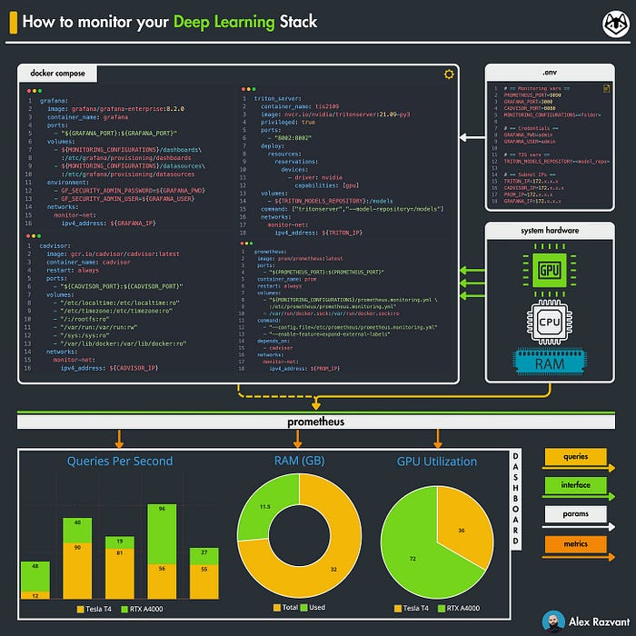
Table of Contents

1. How to set up a performance monitoring pipeline

• Containers
• Configuration Files
• Docker Compose

2. Metrics scrapping configuration

• Adding the Prometheus targets
• Adding the Grafana datasource
• Health check scrapping targets

3. Creating dashboards

• Panels for GPU metrics
• Panels for CPU/RAM metrics

4. Visualizations

Before diving in, let's iterate over the tools that'll be used:

1. Docker is a platform for developing, shipping, and running applications inside lightweight, portable containers — a must for ML Engineers.
2. Docker Compose is a tool for defining and organizing multi-container applications.
3. cAdvisor is an open-source tool developed by Google that provides resource usage and running container performance metrics.
4. Prometheus is a monitoring and alerting toolkit that collects and stores metrics as time-series data, expertise with Prometheus is a big advantage for ML/MLOps Engineers.
5. Grafana is a platform for monitoring and observability, allowing us to create, visualize, alert, and understand metrics of deployed systems. Managing monitoring dashboards is a gold skill for MLOps engineers.
6. Triton Inference Server is a popular model-serving framework developed by NVIDIA, instrumental for deploying complex ML models in production environments. Expertise with Triton is a key skill for MLOps Engineers.

1. Setting up the Docker Compose

Let's start by explaining what each service is doing and preparing the docker-compose to encapsulate and run all these services.

We have the following:

Let's inspect the docker-compose-monitoring.yaml file.

# cat docker-compose-monitoring.yaml
version: '3.4'
services:
  prometheus:
    image: prom/prometheus:latest
    ports:
      - "${PROMETHEUS_PORT}:${PROMETHEUS_PORT}"
    container_name: prometheus
    restart: always
    volumes:
      - "${MONITORING_CONFIGURATIONS}/prometheus.monitoring.yml:/etc/prometheus/prometheus.monitoring.yml"
      - /var/run/docker.sock:/var/run/docker.sock:ro
    command:
      - "--config.file=/etc/prometheus/prometheus.monitoring.yml"
      - "--enable-feature=expand-external-labels"
    depends_on:
      - cadvisor
    networks:
      monitor-net:
        ipv4_address: ${PROM_IP}
  grafana:
    image: grafana/grafana-enterprise:8.2.0
    container_name: grafana
    ports:
      - "${GRAFANA_PORT}:${GRAFANA_PORT}"
    volumes:
      - ${MONITORING_CONFIGURATIONS}/datasources:/etc/grafana/provisioning/datasources
    environment:
      - GF_SECURITY_ADMIN_PASSWORD=${GRAFANA_PWD}
      - GF_SECURITY_ADMIN_USER=${GRAFANA_USER}
    networks:
      monitor-net:
        ipv4_address: ${GRAFANA_IP}
  cadvisor:
    image: gcr.io/cadvisor/cadvisor:latest
    container_name: cadvisor
    restart: always
    ports:
      - "${CADVISOR_PORT}:${CADVISOR_PORT}"
    volumes:
      - "/etc/localtime:/etc/localtime:ro"
      - "/etc/timezone:/etc/timezone:ro"
      - "/:/rootfs:ro"
      - "/var/run:/var/run:rw"
      - "/sys:/sys:ro"
      - "/var/lib/docker:/var/lib/docker:ro"
    networks:
      monitor-net:
        ipv4_address: ${CADVISOR_IP}
  triton_server:
    container_name: tis2109
    image: nvcr.io/nvidia/tritonserver:21.09-py3
    privileged: true
    ports:
      - "8002:8002"
    deploy:
      resources:
        reservations:
          devices:
            - driver: nvidia
              capabilities: [gpu]
    volumes:
      - ${TRITON_MODELS_REPOSITORY}:/models
    command: ["tritonserver","--model-repository=/models", "--strict-model-config=false"]
    networks:
      monitor-net:
        ipv4_address: ${TRITON_IP}
networks:
  monitor-net:
    driver: bridge
    internal: false
    ipam:
        driver: default
        config:
            - subnet: ${SUBNET}
              gateway: ${GATEWAY}

As you may observe, .yaml configuration we have a few ${VAR} that are masked. These are inherited automatically from within a .env file such that this flow follows the best practices on local development and CI/CD pipelines.

Now let's see what's in the .env file:

# == Monitoring vars ==
PROMETHEUS_PORT=9090
GRAFANA_PORT=3000
CADVISOR_PORT=8080
MONITORING_CONFIGURATIONS=<path_to_your_configuration_files> 
# == Credentials ==
GRAFANA_PWD=admin
GRAFANA_USER=admin
# == TIS vars == 
TRITON_MODELS_REPOSITORY=<path_to_your_triton_model_repository>
# == Underlying network ==
SUBNET=172.17.0.0/16
GATEWAY=172.17.0.1
# == Subnet IP's ==
TRITON_IP=172.17.0.3
CADVISOR_IP=172.17.0.4
PROM_IP=172.17.0.5
GRAFANA_IP=172.72.0.6

Pretty much all variables are set, but here are the key 2 we need to take a look at:

1. MONITORING_CONFIGURATIONS This one should point to a folder where you have this structure

.__ monitoring
|  |_ datasources
|  | |_ datasources.yml
|  |_ prometheus.monitoring.yml

1. TRITON_MODEL_REPOSITORY The structure of your model repository should look like this:

model_repository
└── prod_client1_encoder
    └── 1
        └──resnet50.engine
    └── config.pbtxt

The prometheus.monitoring.yml is where we will add the targets (containers) we wish to get metrics from. The datasources.yml is where we'll add Prometheus as a source for Grafana dashboards, such that it will appear when you open Grafana UI.

2. Defining Prometheus scrapping configuration

Let's go ahead and configure the Prometheus targets. We'll write in the prometheus.monitoring.yml file.

global:
  scrape_interval: 15s
  evaluation_interval: 15s
scrape_configs:
  - job_name: 'prometheus'
    static_configs:
      - targets: ['172.17.0.5:9090']
  - job_name: 'triton-server'
    static_configs:
      - targets: ['172.72.0.3:8002']
  
  - job_name: 'cadvisor'
    static_configs:
      - targets: ['172.72.0.4:8080']

We have 3 targets:

1. Prometheus — monitoring Prometheus itself serves as a best practice for healthy monitoring because with thousands of metrics — we might get bottlenecks and it's useful to know the resource usage of Prometheus itself.
2. Triton Server — this one is crucial, as it's at the core of this deep learning stack as it serves and manages our ML models. Triton has an incorporated Prometheus endpoint on port 8002 which offers various metrics across the inference process.
3. cAdvisor — to get CPU/RAM usage across containers in this deployment.

With all these configured, we can start the composer and inspect for any issues. Let's start the containers.

docker compose -f docker-compose-monitoring.yaml up -d

Let's inspect Prometheus targets:

1. Go to your web browser and insert the full Prometheus URL (IP:9090).
2. Go to Status → Targets
3. Check if each target from the scrapping config is healthy (green).

Once we verified these, we could go ahead and create our dashboard in Grafana.

#3 Creating dashboards

To access the Grafana WebUI dashboard, open your browser and go to `localhost:3000`, where 3000 is the port we run the Grafana container.

If you're running this as part of a stack on a cloud deployment or a dedicated server, you can access the web-ui using the public IP of the machine.

If you're prompted to a login page, just use `admin/admin` for the username/password fields. Better security is indeed recommended, but this doesn't fall within the scope of this article.

Once you've opened the Grafana Web, we'll have to do the following:

1. Point the data source to our Prometheus metrics scrapper endpoint
2. Create a new dashboard
3. Add charts to aggregate/visualize metrics we're interested in.

#3.1 Prometheus DataSource

On the left panel, go to the gear icon (settings) and select DataSources. You'll be prompted to a view like this one below:

Click on "Add data source" and under the Time Series Databases select `Prometheus`. As you may have seen, Grafana supports many integrations for metrics scrapping — in this article we'll use Prometheus. You'll be prompted to this view:

Here you'll have to add the URL of your Prometheus endpoint. In our docker-compose deployment, we will use `http://prometheus:9090` following this template `http://container_name:container_port`

If you've reached this point, this section of adding the data source is complete. Let's continue with creating a dashboard.

#3.2 Creating a Grafana Dashboard

On the left panel, go to the "+" sign and select `Dashboard`. You'll be redirected to a new dashboard page with a pre-defined panel group. As we're building everything from scratch, we'll use only `Empty Panels` which we'll set to display key metrics.

Here's the process we'll follow for one example:

1. Add a new query and define the `promql` (Prometheus query language)
2. Configure visualization type, graph style, and legend.

Below is a view of an empty panel:

Next, we'll add a few custom queries to monitor our Triton Inference Server model-serving platform, but first, we should keep in mind the following note:

Since we've decoupled the Inference Process from the actual application code, we have a client-server communication protocol. In order to get an accurate representation of the performance, we have to split the inference timings into these categories: 1. SEND input data from client → server 2. Actual inference on payload (feed-forward) 3. SEND output results from server → client

The first query we'll set will measure the time it took (ms) the model to perform one inference request, considering the number of successful requests. This chart will be a `time-series` since we want to see the progress over time. Here's the query to compose that metric:

(irate(nv_inference_compute_infer_duration_us{job="triton-server"}[$__rate_interval]) / 1000) / irate(nv_inference_request_success{job="triton-server"}[$__rate_interval])

Let's unpack it:

irate: the per-second instant rate of increase of the time series.

nv_inference_compute_infer_duration_us: the time(microseconds) taken to execute the inference, does not include network latency or pre/post-processing.

$__rate_interval: dynamically adjust the rate interval based on the time range selected in the dashboard.

nv_inference_request_success: counts the number of successful inference requests processed.

Below you can see how the query looks.

You might also observe under Legend that we have `{{model}}-{{version}}`. This will filter the chart's legend to display the model + its deployment version within the Triton Server. In this case, we have the model: KeyStone_AIEYE_OBJECTDETECTION_YOLO8M_8003_RTX2080_FP16_CC7.5_v1.0 And version: 1

As per configuring the settings for this new chart, on the right you could specify:

• Chart Type — select either straight/curved/T-step lines
• Metrics Range — select the metric (e.g milliseconds (ms)) and define low_range (e.g 0) and high_range (e.g 100ms)
• Custom Text — to display as legend or other field.

#3.3 Complete Visualization

Based on the flow above, we could create the rest of the charts. Let's add the rest of the panels to compile an entire performance monitoring chart. For the following, create a new panel for each, and fill them with these details:

1. GPU Bytes Used — percentage of VRAM used.

Query: nv_gpu_memory_used_bytes{job="triton-server"}/nv_gpu_memory_total_bytes{job="triton-server"}
Chart Type: Pie
Legend: {{instance}}

2. GPU Utilization — total GPU utilisation

Query: nv_gpu_utilization{job="triton-server"}
Chart Type: Time-series
Legend: NULL

3. Input time/req — time it took the client to send input payload to Triton server.

Query: (irate(nv_inference_compute_input_duration_us{job="triton-server"}[$__rate_interval]) / 1000) / irate(nv_inference_request_success{job="triton-server"}[$__rate_interval])
Chart Type: Time-series
Legend: {{model}}-{{version}}

4. Output time/req — time it took the Server to send output back to client.

Query: (irate(nv_inference_compute_output_duration_us{job="triton-server"}[$__rate_interval]) / 1000)/ irate(nv_inference_request_success{job="triton-server"}[$__rate_interval])
Chart Type: Time-series
Legend: {{model}}-{{version}}

5. DB ratio (#request/#exec) — ratio between successful requests over all requests

Query: sum by (model,version) (rate(nv_inference_request_success{job="triton-server"}[$__rate_interval])/rate(nv_inference_exec_count{job="triton-server"}[$__rate_interval]) )
Chart Type: Time-series
Legend: {{model}}-{{version}}

6. Queue time/request — how long does a request wait in the queue before processed.

Query: sum by (model,version) ((irate(nv_inference_queue_duration_us{job="triton-server"}[$__rate_interval]) / 1000) / irate(nv_inference_request_success{job="triton-server"}[$__rate_interval]))
Chart Type: Time-series
Legend: {{model}}-{{version}}

7. Aggregated Input/Inference/Output — shows IO + inference in a single chart.

Queries:
A: rate(nv_inference_compute_input_duration_us{job="triton-server"}[$__interval]) / 1000
B: rate(nv_inference_compute_infer_duration_us{job="triton-server"}[$__interval]) / 1000
C: rate(nv_inference_compute_output_duration_us{job="triton-server"}[$__interval]) / 1000

Chart Type: Time-series
Legend: {{model}}-{{version}}

Here's the complete dashboard we've created, it showcases:

• GPU VRAM utilization
• Client-to-Server input sending time
• Server inference request time
• Server-to-Client output sending time
• The ratio of success requests/total requests

This kind of dashboard represents a kickstart to monitoring your deployed stack's performance and behavior under stress tests in production.

It provides a concrete way of studying the failure and risk points of your deployments and helps to monitor your SLIs (Service Level Indicators).

You might have seen messages like e.g "99.5% guaranteed up-time" whenever you've accesed any SaaS platform. The 99.5% is an Service Level Agreement(SLA) done between the hosting platform and the client, meaning they assure 99.5% success rate of their platform being up and running.

It can be considered as a confidence indicator.

The Service Level Indicators are metrics monitored, to ensure that the SLAs are respected and the SLOs (Service Level Objectives) are met. The dashboard we've built could, although simple compared to big and complex ones monitoring production stacks, still offer valuable insights towards the goal of meeting the Service Level Agreements.

This also helps planning for a scaling strategy, either adding multiple replicas of the model or scaling up to multiple machines running the Inference Serving framework.

🔗 If you want to read more about SLO/SLI/SLA terms, check them here: https://www.atlassian.com/incident-management/kpis/sla-vs-slo-vs-sli

🔗 Same for key-metrics to monitor your Triton Server Deployment here: https://docs.nvidia.com/deeplearning/triton-inference-server/user-guide/docs/user_guide/metrics.html

Conclusion

In this article, we showcased how to set up and build a performance monitoring stack for our ML Application and Model Serving Framework using Prometheus and Grafana.

Started with preparing the docker-compose file, explaining each step of the workflow, deploying the stack, configuring sources, creating dashboard panels, and ended up with aggregating metrics.

Monitoring is a key part of an MLOps system! Following this tutorial, you'll be able to structure and deploy a monitoring pipeline for your ML application either in testing environments as a single deployment or as an aggregator dashboard (e.g in a cloud scenario setting) to combine multiple input sources and have a single dashboard consumer point from which you monitor the entire stack deployment.

Follow For More!

I'm new on Medium, if you've enjoyed this article make sure to support it by clapping and following me — I'll appreciate it a lot! 🚀

Further Reading

Sorted based on relevance to this article.

In this post you'll learn about how to setup and deploy a MobileNetv2 Image Classification model using the ONNXRuntime engine format and NVIDIA Triton Inference Server. Triton Server is a powerfull framework used widely in production Deep Learning Systems. It goes over all the steps necessary to install, convert the PyTorch model, preparing the config, serve the model and implement the Python client.