In the field of time series forecasting, the architectures of models often rely on either the multi-layer perceptron (MLP) or the Transformer architecture.

MLP-based models, like N-HiTS, TiDE and TSMixer, can achieve very good forecasting performances while remaining fast to train.

On the other hand, Transformer-based models like PatchTST and iTransformer also achieve good performances, but are more memory intensive and require more time to train.

Still, one architecture remains largely underutilized in forecasting: the convolutional neural network (CNN).

Traditionally, CNNs have been applied in computer vision, but their applications in forecasting remains scarce, with only TimesNet being the most recent example.

However, CNNs have been shown to be effective in treating sequential data, and their architecture allow for parallel computation, which can greatly speed up training.

In this article, we thus explore BiTCN, a model proposed in March 2023 in the paper Parameter-efficient deep probabilistic forecasting. By leveraging two temporal convolutional networks (TCN), the model can encode past and future covariates while remaining computationally efficient.

For more details, make sure to read the original paper.

Let's get started!

Explore BiTCN

As mentioned before, BiTCN makes use of two temporal convolutional networks, hence the name BiTCN.

One TCN is responsible to encode future covariates, while the other encodes past covariates and the historical values of the series. That way, the model can learn temporal information from the data, and the use of convolutions keeps it computationally efficient.

There is a lot to dissect here, so let's take a closer look at its architecture.

Architecture of BiTCN

The architecture of BiTCN is composed of many temporal blocks, where each block is made of:

• a dilated convolution
• a GELU activation function
• a dropout step
• a fully-connected layer

The general architecture of a temporal block is shown below.

In the figure above, we can that see that each temporal block generates an output O. The final predictions are obtained by adding all outputs of each block stacked in N layers.

While the dropout and dense layers are common components in neural networks, let's take some time to explore dilated convolutions and the GELU activation function in more detail.

Dilated convolution

To better understand the goal of a dilated convolution, let's remind ourselves of how a default convolution works.

In the figure above, we can see how a typical convolution looks like on a 1D input. The input series is left-padded with zeros to ensure an output of the same length.

Given a kernel size of three and a stride of one, as shown in the figure, the output tensor will also have a length of four.

We can see that each element of the output is dependent on three input values. In other words, the output depends on the value at an index, and the two previous values.

This is what we call the receptive field. Given that we are working with time series data, it would be beneficial to increase the receptive field such that the computation of the output can look at a longer history.

To do so, we can either increase the kernel size, or stack more convolutional layers. Increasing the kernel size is not the best option, as we may lose information and the model may fail to learn useful relationships in the data. So, let's try stacking more convolutions.

From the figure above, we can see that by stacking two convolution operations using a kernel size of three, the last element of the output now depends on five elements of the input. Therefore, the receptive field increased from three to five.

Unfortunately, that also represents a problem, as increasing the receptive field this way will result in very deep networks.

Thus, we use a dilated convolution to increase the receptive field while avoiding adding too many layers to the model.

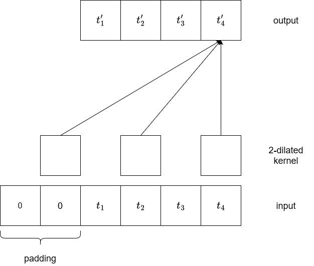
In the figure above, we can see the result of running a 2-dilated convolution. Basically, every two element is considered to generate an output. Therefore, we can see that we now have a receptive field of five without having to stack convolutions.

In practice, to further increase the receptive field, we stack many diluted kernels using a dilation base, usually set to two. This means that the first layer will be a 2¹-dilated kernel, followed by a 2²-dilated kernel, then 2³, and so on.

This way, the receptive field can increase, meaning that the model can consider a longer input sequence to generate the output. By using a dilation base, we can also keep a reasonable number of layers.

Now that we understand the inner workings of dilated convolutions, let's explore the GELU activation function.

GELU activation function

Many deep learning architectures employ the Rectified Linear Unit or ReLU activation function. The equation of ReLU is shown below.

From the equation above, we can see that ReLU simply takes the maximum value between zero and the input. In other words, if the input is positive, the input is returned. If the input is negative, zero is returned.

While ReLU helps alleviate the problem of vanishing gradients, it can also create what is called the Dying ReLU problem.

This happens when certain neurons in the network only output zeros, meaning that they do not contribute to the model's learning anymore.

To counter that situation, the Gaussian Error Linear Unit or GELU can be used. The GELU equation is shown below.

With this function, the activation function allows for small negative values when the input is smaller than zero.

That way, neurons are less likely to die out, because non-zero values can be returned with negative inputs. This gives a richer gradient for backpropagation, and we can keep the integrity of the model's capability.

Putting it all together in BiTCN

Now that we understand the inner workings of a temporal block in BiTCN, let's see how it all comes together in the model.

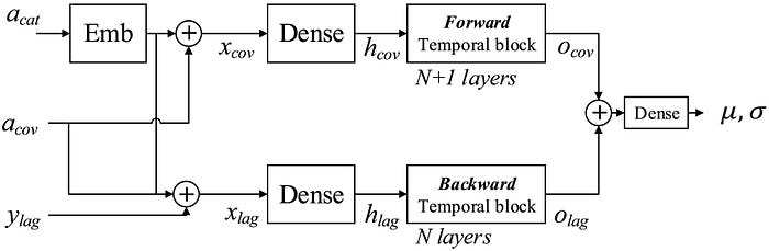
In the figure above, we can see that lagged values are combined with all past covariates before being sent through a dense layer, and through a stack of temporal blocks.

On the top, we also see categorical covariates being embedded first, before being combined with other covariates. Note that here, both past and future covariates are combined as shown below.

Then, they are led through a dense layer, and a stack of temporal blocks.

The output is then the combination of information coming from lagged values and from the covariates as shown below.

The figure above really emphasizes the idea that one temporal block is using the future values of covariates (shown as red dots) to inform the output of the model (shown as yellow dots).

Finally, BiTCNemploys a Student's t-distribution to construct confidence intervals around the predictions.

Now that we understand the inner workings of BiTCN, let's apply it in a small forecasting project using Python.

Forecasting with BiTCN

For this experiment, we apply BiTCN along with N-HiTS and PatchTST on a long-horizon forecasting task.

Specifically, we use it to forecast the daily views of a blog website. The dataset contains the daily number of views, and exogenous features like an indicator for the day a new article is published, and an indicator for US holidays.

I compiled this dataset myself using the traffic on my own website. The dataset is publicly available here.

For this portion, we use the library neuralforcast, as this is the only library, to my knowledge, that provides a ready-to-use implementation of BiTCN with support of exogenous features.

As always, the full source code for this experiment is on GitHub.

Let's get started!

Initial setup

The natural first step is to import the required libraries for this project.

import pandas as pd
import numpy as np
import matplotlib.pyplot as plt

from neuralforecast.core import NeuralForecast
from neuralforecast.models import NHITS, PatchTST, BiTCN

Then, we read the data into a DataFrame.

df = pd.read_csv('https://raw.githubusercontent.com/marcopeix/time-series-analysis/master/data/medium_views_published_holidays.csv')
df['ds'] = pd.to_datetime(df['ds'])

Optionally, we can plot the data.

published_dates = df[df['published'] == 1]
holidays = df[df['is_holiday'] == 1]

fig, ax = plt.subplots(figsize=(12,8))

ax.plot(df['ds'], df['y'])
ax.scatter(published_dates['ds'], published_dates['y'], marker='o', color='red', label='New article')
ax.scatter(holidays['ds'], holidays['y'], marker='x', color='green', label='US holiday')
ax.set_xlabel('Day')
ax.set_ylabel('Total views')
ax.legend(loc='best')

fig.autofmt_xdate()

plt.tight_layout()

From the figure above, we can clearly see a weekly seasonality, with more visits occurring during weekdays than during the weekend.

Also, spikes in visits usually follow new articles being published (shown as red dots), as new content usually drives more traffic. Finally, we see that US holidays (labelled by green crosses) often signal lower traffic.

Thus, we can see that this is a series with clear influences from exogenous features, making it a great use case for BiTCN.

Data processing

Now, let's split the data into a train and test set. We reserve the last 28 entries for testing.

train = df[:-28]
test = df[-28:]

Then, we create a DataFrame containing the dates for our forecast horizon, as well as the future values of the exogenous variables.

Note that providing the future values of exogenous variables makes sense, as future US holidays' dates are known in advance, and the publishing of an article can also be planned.

future_df = test.drop(['y'], axis=1)

Great! We are now ready to model our series.

Modeling

As mentioned, we use N-HiTS (MLP-based), BiTCN (CNN-based) and PatchTST (Transformer-based) for this project.

Note that N-HiTS and BiTCN both support modeling with exogenous features, but not PatchTST.

Again, the horizon for this experiment is set to 28, as this covers the entire length of our test set.

horizon = len(test)

models = [
    NHITS(
        h=horizon,
        input_size = 5*horizon,
        futr_exog_list=['published', 'is_holiday'],
        hist_exog_list=['published', 'is_holiday'],
        scaler_type='robust'),
    BiTCN(
        h=horizon,
        input_size=5*horizon,
        futr_exog_list=['published', 'is_holiday'],
        hist_exog_list=['published', 'is_holiday'],
        scaler_type='robust'),
    PatchTST(
        h=horizon,
        input_size=2*horizon,
        encoder_layers=3,
        hidden_size=128,
        linear_hidden_size=128,
        patch_len=4,
        stride=1,
        revin=True,
        max_steps=1000
    )
]

Then, we simply fit our models on the training set.

nf = NeuralForecast(models=models, freq='D')
nf.fit(df=train)

Then, we can generate predictions using the future values of our exogenous features.

preds_df = nf.predict(futr_df=future_df)

Excellent! At this point, we have predictions stores in preds_df . We can evaluate the performance of each model.

Evaluation

We start off by joining the predictions and the actual values in a single DataFrame.

test_df = pd.merge(test, preds_df, 'left', 'ds')

Optionally, we can plot the predictions against the actual values, resulting in the figure below.

In the figure above, we can see that all models seem to have globally over-predicted the actual traffic.

Let's then measure the mean absolute error (MAE) and symmetric mean absolute percentage error (sMAPE) to find the best performing model.

from utilsforecast.losses import mae, smape
from utilsforecast.evaluation import evaluate

evaluation = evaluate(
    test_df,
    metrics=[mae, smape],
    models=["NHITS", "BiTCN", "PatchTST"],
    target_col="y",
)

evaluation = evaluation.drop(['unique_id'], axis=1)
evaluation = evaluation.set_index('metric')

evaluation.style.highlight_min(color='blue', axis=1)

From the table above, we can see that BiTCN achieves the best performance, since the MAE and sMAPE are the lowest for this model.

While this experiment alone is not a robust benchmark of BiTCN, it is interesting to see it achieve the best results in a context of forecasting with exogenous features.

Conclusion

The BiTCN model makes use of two temporal convolutional networks to encode both past values and future values of covariates for efficient multivariate time series forecasting.

It is interesting to see successful application of convolution neural networks in the field of time series, as most models are MLP-based or Transformer-based.

In our small experiment, BiTCN achieved the best performance, but I firmly believe that every problem requires its unique solution, and now you can add BiTCN to your toolbox and apply it in your projects.

Thanks for reading! I hope that you enjoyed it and that you learned something new!

Learn the latest time series analysis techniques with my free time series cheat sheet in Python! Get the implementation of statistical and deep learning techniques, all in Python and TensorFlow!

Cheers 🍻

Support me

Enjoying my work? Show your support with Buy me a coffee, a simple way for you to encourage me, and I get to enjoy a cup of coffee! If you feel like it, just click the button below 👇

References

Parameter-efficient deep probabilistic forecasting by Olivier Sprangers, Sebastian Schelter, Maarten de Rijke

Explanation of dilated convolution and figures of dilates convolutions inspired: Temporal convolutional networks and forecasting by Unit8