

1. What is XGBoost?
- Full Name: eXtreme Gradient Boosting
- Creator: Tianqi Chen (Ph.D., University of Washington)
- Foundation: Built on Gradient Boosting Decision Trees (GBDT)
- Category: Iterative boosting, tree-based algorithm
- Application Scope: Suitable for both classification and regression tasks
Advantages:
- Fast execution speed
- High predictive performance
- Capable of handling large-scale datasets
- Supports multiple programming languages
- Allows custom loss functions
Disadvantages:
- Relatively new (released in 2014)
- Limited adoption in industrial applications
- Still undergoing validation and testing
2. Basic Knowledge: GBDT
XGBoost is an improvement of the boosting algorithm based on GBDT (Gradient Boosting Decision Trees). It internally uses regression trees as the decision trees.
Regression Tree Splitting Nodes For a squared loss function, the regression tree fits the residuals. For a general loss function (using gradient descent), it fits the approximate values of the residuals.
When splitting nodes, the algorithm enumerates all possible feature values to select the best split point.
The final prediction result is the sum of the predictions from all trees.
3. Understanding the XGBoost Algorithm
3.1 Definition of Tree Complexity
Tree complexity in XGBoost is defined by evaluating factors such as the structure of the tree, the number of leaf nodes, and regularization terms to prevent overfitting. This complexity plays a crucial role in model optimization and performance tuning.
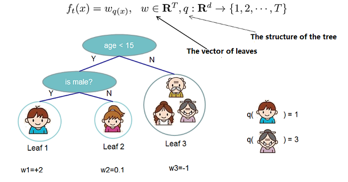
Split the tree into the structure part (q) and the leaf weight part (w).
The tree complexity function and example:
The reason for defining the structure and complexity of trees is simple: it allows us to measure the complexity of the model, which can effectively control overfitting.
3.2 Boosting Tree Models in XGBoost
Like traditional boosting tree models, the boosting model in XGBoost also uses residuals (or the negative gradient direction). The difference is that when selecting the split nodes, it is not necessarily the minimum squared loss.
3.3 Rewrite of the Objective Function
The final objective function only depends on the first and second derivatives of the error function for each data point. The reason for writing it this way is obvious: during the optimization process of the previous objective function, it was convenient to solve for the squared loss function, but for other loss functions, it became quite complicated. Through the transformation using the second-order Taylor expansion, solving for other loss functions becomes feasible. Very impressive! Once the split candidate set is defined,
the objective function can be further modified. The candidate set for splitting nodes is a crucial step, and it is the key to XGBoost's fast performance. How this set is selected will be introduced later.
Solve:
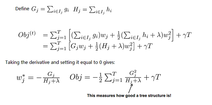
3.4 Scoring Function for Tree Structure
Obj represents the maximum reduction in the objective when a tree structure is specified. (structure score)
For each attempt to add a split to an existing leaf
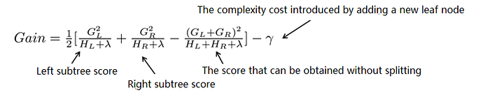
This way, during the tree-building process, it is possible to dynamically decide whether to add a node.
Assuming we need to enumerate conditions such as x<ax < a, for a specific split aa, we need to calculate the sum of the derivatives on the left and right sides of aa. For all possible values of aa, we can enumerate the gradient sums GLGL and GRGR for all splits by doing a single left-to-right scan. Then, we can calculate the score for each split option using the formula above.
3.5 Finding the Candidate Set for Split Nodes
- Brute Force Enumeration
- Approximation Method The approximation method determines a set of candidate split points based on the distribution of features, using percentages. The optimal split point is found by traversing all candidate split points. Two strategies: Global strategy and Local strategy.
- In the global strategy, a global set of candidate split points is determined for each feature and does not change.
- In the local strategy, a split point must be reselected for each split. The global strategy requires a larger split set, while the local strategy can use a smaller one. Comparing the supplementary candidate set strategy with the number of split points and their impact on the model: the global strategy requires finer split points to achieve similar results as the local strategy.
3. Weighted Quantile Sketch
For the k-th feature, construct the dataset Dk = (x1k, h1), (x2k, h2),…, (xnk, hn)
hi is the second-order gradient of the loss function corresponding to this data point.
Define the sequence function as a weighted sequence function.
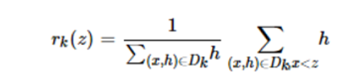
The above formula represents the proportion of samples where the k-th feature is less than z.
The goal of the candidate set is to ensure that the difference between two adjacent candidate split points does not exceed the threshold ɛ.

Tianqi Chen proposed and proved, from a probabilistic perspective, a weighted distributed Quantile Sketch.
4. Summary of XGBoost Improvements
- The objective function is approximated using a second-order Taylor expansion.
- The complexity of the tree is defined and applied to the objective function.
- Split nodes grow dynamically through structure scoring and split loss.
- The candidate set for split nodes is obtained using a distributed Quantile Sketch.
- It can handle sparse and missing data.
- Feature column sampling is used to prevent overfitting.
5. XGBoosting Case: Financial Fraud Detection Model
Credit card fraud usually occurs when a cardholder's information is stolen and the card is copied for transactions, or when a credit card is activated and used by someone else after being fraudulently claimed. Once fraud occurs, both the cardholder and the bank incur financial losses. Therefore, building a financial fraud detection model using big data technology is crucial for banks.
5.1 Model Building
XGBoost can be used for both classification and regression analysis, with corresponding models being the XGBoost classification model (XGBClassifier) and XGBoost regression model (XGBRegressor).
Here, we will demonstrate using the classification model as an example.
5.1.1 Reading Data
The following code reads 1,000 customer credit card transaction records.
The feature variables include the number of device changes by the customer, the number of payment failures before the current transaction, the number of IP changes, the number of countries of IP changes, and the amount of the current transaction.
The target variable is whether the current transaction is fraudulent. A transaction that results from credit card fraud is marked as 1 (fraud), and a normal transaction is marked as 0.
There are 400 fraud samples and 600 non-fraud samples.
import pandas as pd
df = pd.read_excel('credit_card_transaction.xlsx')
df.head()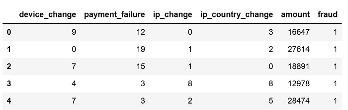
5.1.2 Feature Variable and Target Variable Extraction, Dataset and Test Set Splitting
X = df.drop(columns='fraud')
y = df['fraud']

from sklearn.model_selection import train_test_split
X_train,X_test,y_train,y_test = train_test_split(X,y,test_size=0.2,random_state=123)
5.1.3 Model Building and Training
from xgboost import XGBClassifier
model = XGBClassifier(n_estimators = 100, learning_rate = 0.05)
model.fit(X_train, y_train)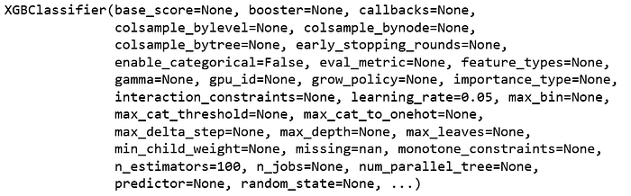
The second line of code assigns the XGBClassifier() to the variable model and sets the maximum number of iterations for the weak learners (or the number of weak learners) with the n_estimators parameter to 100, and the weight shrinkage coefficient for the weak learners, learning_rate, to 0.05. The other parameters are set to their default values.
5.2 Model Prediction and Evaluation
After the model is built, the following code is used to make predictions on the test set data.
y_pred = model.predict(X_test)
y_pred
The following code can be used to summarize the predicted values and actual values for comparison.
a = pd.DataFrame()
a['prediction'] = list(y_pred)
a['practical'] = list(y_test)
a.head()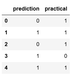
As you can see, the prediction accuracy for the first 5 items is 40%. The following code can be used to view the prediction accuracy for all the test set data.
from sklearn.metrics import accuracy_score
accuracy_score(y_test, y_pred)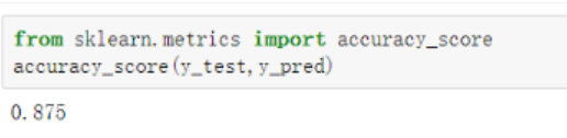
The XGBoost classification model essentially does not predict the exact 0 or 1 classification, but rather predicts the probability that a sample belongs to a certain class. You can use the predict_proba() function to view the predicted probabilities for each class. The code is as follows.
y_pred_proba = model.predict_proba(X_test)
y_pred_proba[:,1]
The obtained y_pred_proba is a two-dimensional array, where the first column represents the probability of the classification being 0 (i.e., non-fraud), and the second column represents the probability of the classification being 1 (i.e., fraud). The above shows how to view the probability of fraud (classification 1).
Next, we evaluate the model's prediction performance by plotting the ROC curve. The code is as follows.
from sklearn.metrics import roc_curve
fpr,tpr,thres = roc_curve(y_test, y_pred_proba[:,1])

import matplotlib.pyplot as plt
plt.plot(fpr,tpr)
plt.xlabel('fpr')
plt.ylabel('tpr')
plt.show()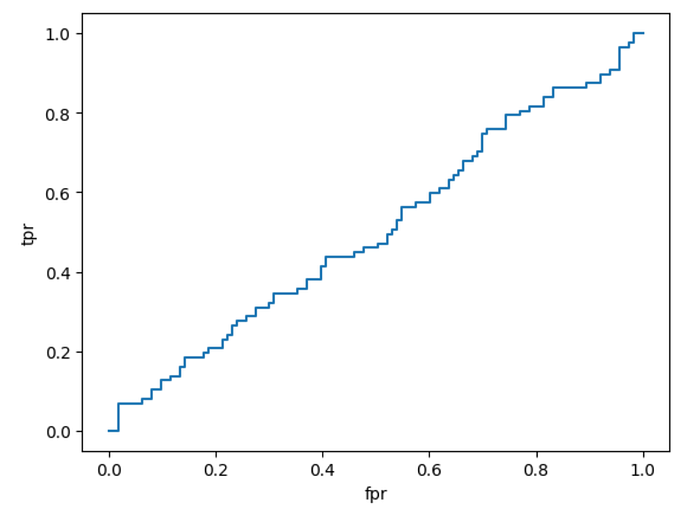
The following code calculates the AUC value of the model.
from sklearn.metrics import roc_auc_score
roc_auc_score(y_test, y_pred_proba[:,1])
The following code allows you to view the feature importance of each feature variable, helping to identify the most important features in determining credit card fraud behavior.
a = pd.DataFrame()
a['feature'] = X.columns
a['feature_importance'] = model.feature_importances_
a.sort_values('feature_importance', ascending=False)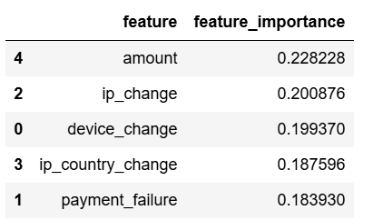
5.3 Model Parameter Tuning
Use GridSearch for hyperparameter tuning.
from sklearn.model_selection import GridSearchCV
parameters = {'max_depth':[1,3,5],'n_estimators':[50,100,150],'learning_rate':[0.01,0.05,0.1,0.2]}
model = XGBClassifier()
grid_search = GridSearchCV(model,parameters,scoring='roc_auc',cv=5)
grid_search.fit(X_train,y_train)
grid_search.best_params_

# best parameters
# {'learning_rate': 0.1, 'max_depth': 3, 'n_estimators': 150}
From the above results, it can be seen that for the data in this case, the best prediction performance of the model is achieved when the maximum depth of the weak learner decision tree is limited to 3, the maximum number of iterations for the weak learners is set to 150, and the weight shrinkage coefficient for the weak learners is set to 0.1.
Thank you for reading.