MACHINE LEARNING

A Recurrent Neural Network (RNN) is one of the most used deep-learning algorithms for sequence processing. The difference between an RNN and a feedforward neural network is that the former one can 'memorize' the chronological information in a sequence while the later one processes the entire sequence in one go.

Therefore, we'd better use RNN when the chronological order of the data is important for the issue, such as time-series data analysis or natural language processing (NLP).

However, it is still under debate whether a player's previous games can affect the result of the coming game. So, I would like to explore whether RNN is a good fit for the game prediction problem on the basketball court.

In this short article, I am trying to use a deep-learning model to predict LeBron James's future game results based on the game stats and results of the previous ones.

The Dataset

I scraped the game stats of LeBron's 1,258 games from Season 2003–04 to Season 2019–20 with Python. For those who are interested in the scraping procedure, please refer to one of my previous posts.

Here is how the data looks.

In another post of mine, I have shown that "GmSc" (player's game score), "+/-" (plus/minus metric), and "Minutes" (played minutes) are three of the most important features in explaining the corresponding game result. So, to reduce the input data dimension, I only keep these game stats as well as the game results ("Win") in our model. For each data point, I extract the past 10 games' stats (t-9, t-8, …, t-1, t) and the aim is to predict the game result of the next game (t + 1).

I use the first 800 games as our training data, the next 300 games as the validation data, and the last 158 games as the test data.

The entire pre-processing of the data is shown below.

data_u = df[["GmSc","+/-","Minutes","Win"]].to_numpy()
mean = data_u[:800].mean(axis=0)
data_u -= mean
std = data_u[:800].std(axis=0)
data_u /= std

The normalization parameters (mean and standard deviation) are generated from the training data only (first 800 games) and then the parameters are applied to the entire dataset.

Loading the entire dataset is very memory consuming, sometimes even impossible. So feeding data to the model using a data generator (implemented in Keras) is a good choice to deal with the issue. Even though here I have a very small (1,258 data points) dataset, I would still like to use a data generator in my pipeline, which will benefit the future extension.

def generator(data, lookback, delay, start, end, batch_size = 64):
    if end is None:
        end = len(data) - delay - 1
    i = start + lookback
    while True:
        if i + batch_size >= end:
            i = start + lookback
        rows = np.arange(i, min(i + batch_size, end))
        i += len(rows)
        samples = np.zeros((len(rows),
                           lookback,
                           data.shape[-1]))
        res_s = np.zeros((len(rows),))
        
        for j, row in enumerate(rows):
            indices = range(rows[j] - lookback, rows[j])
            samples[j] = data[indices]
            tar_v = data[rows[j] + delay][3]
            if tar_v > 0:
                res_s[j] = 1
            else:
                res_s[j] = 0
        yield samples, res_s

I set lookback as 10, which means using the 10 previous games as the input. I set delay as 1, which means predicting the next game result.

lookback = 10
delay = 1
batch_size = 128
steps_per_epc = int(800/batch_size)

To define the train, validation, and test data generator, I just need to feed the start and end value to the generator function.

train_generator = generator(data_u,
                           lookback = lookback,
                           delay = delay,
                           start = 0,
                           end = 800,
                           batch_size = batch_size)
val_generator = generator(data_u,
                           lookback = lookback,
                           delay = delay,
                           start = 801,
                           end = 1100,
                           batch_size = batch_size)
test_generator = generator(data_u,
                           lookback = lookback,
                           delay = delay,
                           start = 1101,
                           end = None,
                           batch_size = batch_size)

Correspondingly, I need to specify the number of steps needed to go over the validation and test dataset.

val_steps = (1100 - 801 - lookback)
test_steps = (len(data_u) - 1101 - lookback)

Next, I am going to build model structures.

The Modeling Results

To start with, I build an ANN with densely connected layers as my baseline model to compare my other models with.

from keras.models import Sequential
from keras import layers
from keras.optimizers import RMSprop
model_ann = Sequential()
model_ann.add(layers.Flatten(input_shape = (lookback, data_u.shape[-1])))
model_ann.add(layers.Dense(32,activation = 'relu'))
model_ann.add(layers.Dropout(0.3))
model_ann.add(layers.Dense(1,activation = 'sigmoid'))
model_ann.summary()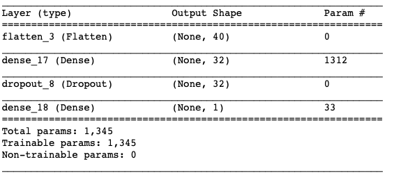

Then, I compile the model and record the fitting process.

model_ann.compile(optimizer = RMSprop(lr = 1e-2),
                 loss = 'binary_crossentropy',
                 metrics = ['acc'])
history = model_ann.fit_generator(train_generator,
                                  steps_per_epoch=steps_per_epc,
                              epochs = 20, 
                              validation_data = val_generator,
                              validation_steps = val_steps)

To check the performance on the validation dataset, I plot the loss curve.

acc_ = history_dic['loss']
val_acc_ = history_dic['val_loss']
epochs = range(1,21)
#plt.clf()
plt.plot(epochs,acc_, 'bo', label = "training loss")
plt.plot(epochs, val_acc_, 'r', label = "validation loss")
plt.xlabel('Epochs')
plt.ylabel('loss')
plt.legend()
plt.show()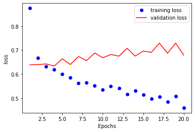

As expected, the model becomes overfitting after several epochs. To evaluate the model objectively, I apply it to the test set and get accuracy as 60%.

scores = model_ann.evaluate_generator(test_generator,test_steps) 
print("Accuracy = ", scores[1]," Loss = ", scores[0])

Next, I implement an RNN by using one LSTM layer followed by two densely connected layers.

model_rnn = Sequential()
model_rnn.add(layers.LSTM(32,
                        dropout=0.2,
                        recurrent_dropout=0.2,
                        input_shape=(None,data_u.shape[-1])))
model_rnn.add(layers.Dense(32,activation = 'relu'))
model_rnn.add(layers.Dropout(0.3))
model_rnn.add(layers.Dense(1,activation='sigmoid'))
model_rnn.summary()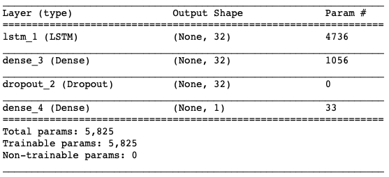

The model training is similar to that of ANN above.

model_rnn.compile(optimizer = RMSprop(lr = 1e-2),
                 loss = 'binary_crossentropy',
                 metrics = ['acc'])
history = model_rnn.fit_generator(train_generator, 
                                  steps_per_epoch=steps_per_epc,
                              epochs = 20, 
                              validation_data = val_generator,
                              validation_steps = val_steps)

The training and validation set performance is as below.

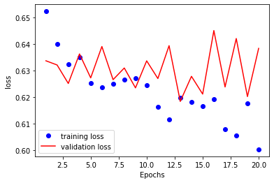
The overfitting is not as severe as that of the ANN. I also evaluate the model on the test data, which yields an accuracy of 62.5%. Even though the performance on the test set is better than that of the ANN with densely connected layers, the improvement is tiny.

To gain better performance, I try to increase the complexity of the model by adding one more recurrent layer. However, to reduce the computational cost, I replace the LSTM layer by the Gated Recurrent Unit (GRU). The model is shown below.

model_rnn = Sequential()
model_rnn.add(layers.GRU(32,
                        dropout=0.2,
                        recurrent_dropout=0.2,
                         return_sequences = True,
                        input_shape=(None,data_u.shape[-1])))
model_rnn.add(layers.GRU(64, activation = 'relu',dropout=0.2,recurrent_dropout=0.2))
model_rnn.add(layers.Dense(32,activation = 'relu'))
model_rnn.add(layers.Dropout(0.3))
model_rnn.add(layers.Dense(1,activation = 'sigmoid'))
model_rnn.summary()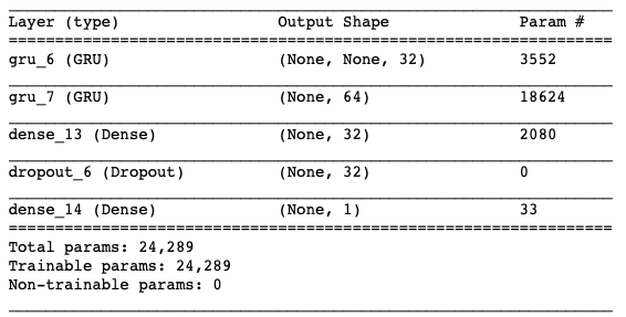

The training and validation set performance is as below.

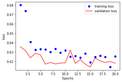
No serious overfitting is detected on the plot. Even though the accuracy of the test data has increased to 64%, the improvement is still tiny. I begin to doubt whether RNN can do the job.

However, I give my last try by further increasing the complexity of the model. Specifically, I enable the recurrent layer to be bidirectional.

model_rnn = Sequential()
model_rnn.add(layers.Bidirectional(layers.GRU(32,
                        dropout=0.2,
                        recurrent_dropout=0.2,
                         return_sequences = True),
                        input_shape=(None,data_u.shape[-1])))
model_rnn.add(layers.Bidirectional(layers.GRU(64, activation = 'relu',dropout=0.2,recurrent_dropout=0.2)))
model_rnn.add(layers.Dense(32,activation = 'relu'))
model_rnn.add(layers.Dropout(0.3))
model_rnn.add(layers.Dense(1,activation='sigmoid'))
model_rnn.summary()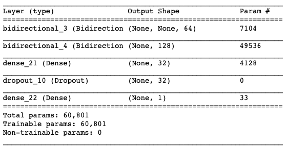

This time, the training and validation set performance is as below.

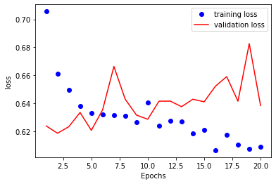
Actually, before the model starts overfitting, there is not much difference between this model and the previous one on the validation loss. The accuracy of the test set is 64% as well.

By exploring all the models above, I kind of realize that the RNN may not be a good fit for the NBA game result prediction problem. There are indeed tens of hyperparameters that can be tuned, the difference between the ANN and RNN, however, is too small.

Diagnose of The Data

I don't want to be fooled by the value of the test set accuracy, so I further diagnose the data set to check whether the models really work.

I check LeBron's James winning rate in the training, validation, and testing datasets.

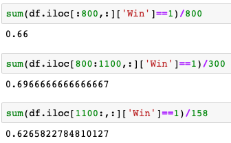
Oops! The winning rate in the test dataset is 62.7%, which means if I guess that LeBron will win all the games, I still get 62.7% accuracy.

These results suggest that my models are no better than random guessing. Sad…

Maybe I haven't explored the hyperparameter space comprehensively, or maybe LeBron's games are not predictable. But one thing is for sure, ~1000 data points are far from sufficient.

Discussions

In this article, I showed an example of developing failing models for the game results prediction problem. In case you think you've learned nothing from it, I would like to force myself to list some takeaways. At least you might meet some of these details in your modeling.

1. It's important to push the model towards overfitting first because a model with weak representation power will never address the problem.
2. If your model is still underfitting after a large number of epochs, say 40, probably you need to increase the learning rate.
3. Nothing will be fancy if you are only exposed to a limited amount of data. Your complex model could be worse than random guessing.

References:

1. François Chollet. Deep Learning with Python.
2. Basketball Reference.

Thanks for your time. If you enjoyed reading the article, please follow me on Medium. Here are some of my previous articles.