
There are various strategies for selecting stocks, one of which is to buy stocks at new prices. While many investors would like to buy stocks at the lowest possible price, this strategy buys stocks at the highest price. In this article, we will consider stock selection based on this strategy and show that his strategy can help you find the most attractive stocks.
import os
import glob
import pandas as pd
import matplotlib.pyplot as plt
import datetime as dt
from concurrent import futures
import numpy as np
from scipy.stats import gaussian_kde
import pandas_datareader.data as web
data_dir = "./data/stock_data_for_finding_attractive_stocks"
os.makedirs(data_dir, exist_ok=True)
Download Dataset
Pandas has a read_html method that can read table data from a web page. In this example, we will use the read_html method to retrieve information about the S&P500 from Wikipedia. There are two tables in the wiki page; S&P 500 component stocks and selected changes to the list of S&P 500 components.
I recommend that you keep a list of stocks in the S&P 500 along with the date of acquisition, as there are about 20 stocks that are replaced annually. For more information, please read my previous article; Data Analysis of S&P500 stocks in Python -investment strategy during post-pandemic-.
tables = pd.read_html('https://en.wikipedia.org/wiki/List_of_S%26P_500_companies')
sp500_df = tables[0]
second_table = tables[1]
print(sp500_df.shape)
sp500_df["Symbol"] = sp500_df["Symbol"].map(lambda x: x.replace(".", "-"))  # rename symbol to escape symbol error
sp500_df.to_csv("./data/SP500_20220430.csv", index=False)
sp500_df = pd.read_csv("./data/SP500_20220430.csv")
print(sp500_df.shape)
sp500_tickers = list(sp500_df["Symbol"])
sp500_df.head()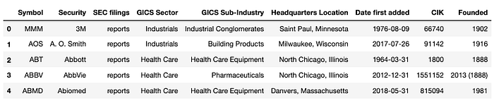
def download_stock(stock):
    try:
        print(stock)
        stock_df = web.DataReader(stock,'yahoo', start_time, end_time)
        stock_df['Name'] = stock
        output_name = f"{data_dir}/{stock}.csv"
        stock_df.to_csv(output_name)
    except:
        bad_names.append(stock)
        print('bad: %s' % (stock))
""" set the download window """
start_time = dt.datetime(1900, 1, 1)
end_time = dt.datetime(2022, 4, 30)
bad_names =[] #to keep track of failed queries
#set the maximum thread number
max_workers = 20
now = dt.datetime.now()
path_failed_queries = f'{data_dir}/failed_queries.txt'
if os.path.exists(path_failed_queries):
    with open(path_failed_queries) as f:
        failed_queries = f.read().split("\n")[:-1]
        sp500_tickers_ = failed_queries
else:
    sp500_tickers_ = sp500_tickers
print("number of stocks to download:", len(sp500_tickers_))
workers = min(max_workers, len(sp500_tickers_)) #in case a smaller number of stocks than threads was passed in
with futures.ThreadPoolExecutor(workers) as executor:
    res = executor.map(download_stock, sp500_tickers_)
""" Save failed queries to a text file to retry """
if len(bad_names) > 0:
    with open(path_failed_queries, 'w') as outfile:
        for name in bad_names:
            outfile.write(name+'\n')
finish_time = dt.datetime.now()
duration = finish_time - now
minutes, seconds = divmod(duration.seconds, 60)
print(f'The threaded script took {minutes} minutes and {seconds} seconds to run.')
print(f"{len(bad_names)} stocks failed: ", bad_names)
Preprocessing data
No significant data preprocessing is performed this time. We will only obtain the date of the highest price.
historical_stock_data_files = glob.glob(f"./{data_dir}/*.csv")
highest_day_list = []
for files in historical_stock_data_files:
    price = pd.read_csv(files, index_col="Date", parse_dates=True)
    ticker = os.path.splitext(os.path.basename(files))[0]
price_close = price[["Close"]]
    highest_day = price_close.idxmax()[0]
    highest_price = price_close.max()[0]
    highest_day_list.append(
        pd.DataFrame({"highest_day": [highest_day], "ticker": [ticker], "highest_price": highest_price}))

df = pd.concat(highest_day_list).reset_index(drop=True)
print(df.shape)
df.head()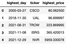
# additional info
df["highest_month"] = df["highest_day"].dt.to_period("M")
df = pd.merge(df, sp500_df[["Symbol", "GICS Sector", "GICS Sub-Industry"]], left_on='ticker', right_on='Symbol')
Exploratory Data Analysis
Let's take a look at some of the stocks that have recently reached new highs.
df.sort_values("highest_day",ascending=False).head(20)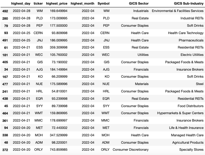
Surprisingly, many stocks have recently reached new highs, although they may not necessarily be well-known stocks. These stocks that have just recently made new prices may be attractive because most of the investors who bought them are making money, so selling pressure is likely to be weak.
Let's break down the highest-priced stocks in April this year by industry.
industry_value_counts = df[df["highest_day"] >= "2022-04-01"]["GICS Sub-Industry"].value_counts()
fig, ax = plt.subplots(figsize=(20, 8))
ax.bar(industry_value_counts.index, industry_value_counts.values)
ax.set_xticklabels(industry_value_counts.index, rotation=90)
ax.set_xlabel("industry")
ax.set_ylabel("number of stocks")
plt.show()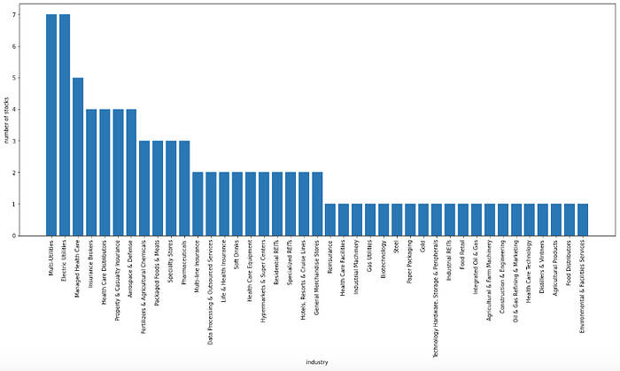
Multi-utilities and electric utilities accounted for seven stocks each, followed by managed health care.
Since there seem to be some common words, let's extract only those that contain specific keywords. It was hard to tell from the bar chart alone, but it seems that many industries include words such as utilities, health care, and insurance.
display(industry_value_counts[industry_value_counts.index.str.contains("Utilities")])
display(industry_value_counts[industry_value_counts.index.str.contains("Health Care")])
display(industry_value_counts[industry_value_counts.index.str.contains("Insurance")])
So what about the other months? Let's take a look at when the components of the S&P 500 hit their highs.
highest_day_count = df.groupby("highest_month").count()
highest_day_count["ticker"].plot()
plt.title("Number of stocks that reached new highs")
plt.ylabel("number of stocks")
plt.show()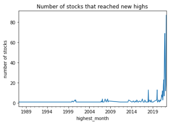
Since many of the stocks seem to have reached their highest prices within the last few years, we will cut out the portion after 2021.
highest_day_count["ticker"].plot(marker=".")
plt.grid(axis='y')
plt.title("Number of stocks that reached new highs")
plt.xlim("2021-01-01","2022-04-30")
plt.ylabel("number of stocks")
plt.show()
Interestingly, the largest number of highest-priced stocks was in April of this year; 87 of the 504 stocks took the highest price this April.
The next largest peak was last December with 69 stocks.
The total number of stocks that have failed to reach new highs since the beginning of this year is 356 (71% of S&P500 stocks).
Let's check the highest price days of popular growth stocks.
tikcer_list = ["GOOG", "AAPL", "FB", "AMZN", "MSFT", "TSLA", "NVDA"]
df[df["ticker"].isin(tikcer_list)]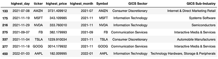
These popular technology stocks(other than APPL) have been unable to rise after reaching their highs last year.
As before, let's look at the industry classification of the 356 stocks that reached their highest price last year or earlier.
industry_value_counts = df[df["highest_day"] <= "2021-12-31"]["GICS Sub-Industry"].value_counts()
fig, ax = plt.subplots(figsize=(20, 8))
ax.bar(industry_value_counts.index, industry_value_counts.values)
ax.set_xticklabels(industry_value_counts.index, rotation=90)
ax.set_xlabel("industry")
ax.set_ylabel("number of stocks")
plt.show()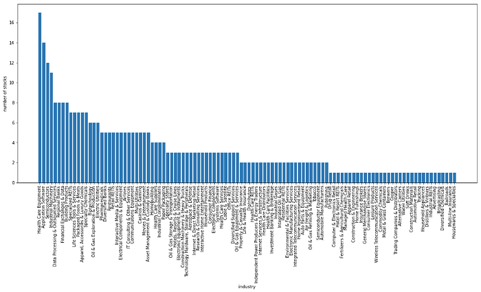
This time, health care equipment topped the list with 17 stocks, followed by application software with 14 and semiconductors with 12.
Finally, for comparison, we plot the number of stocks that reached a high last year or earlier (in orange) and the number of stocks that reached a high this year (in blue) as a stacked bar chart for each industry.
df["in_2022"] = df["highest_day"].map(lambda x: False if x.year < 2022 else True)
value_counts_before_2022 = df[df["in_2022"]==False]["GICS Sub-Industry"].value_counts()
value_counts_2022 = df[df["in_2022"]==True]["GICS Sub-Industry"].value_counts()
value_counts_before_2022.name = "~2021"
value_counts_2022.name = "2022"
comparison_df = pd.concat([value_counts_2022, value_counts_before_2022], axis=1)
comparison_df = comparison_df.fillna(0)
comparison_df.head()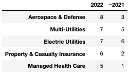
fig, ax = plt.subplots(figsize=(20, 8))
comparison_df.plot(kind='bar', stacked=True, ax=ax)
ax.set_xlabel("industry")
ax.set_ylabel("number of stocks")
plt.show()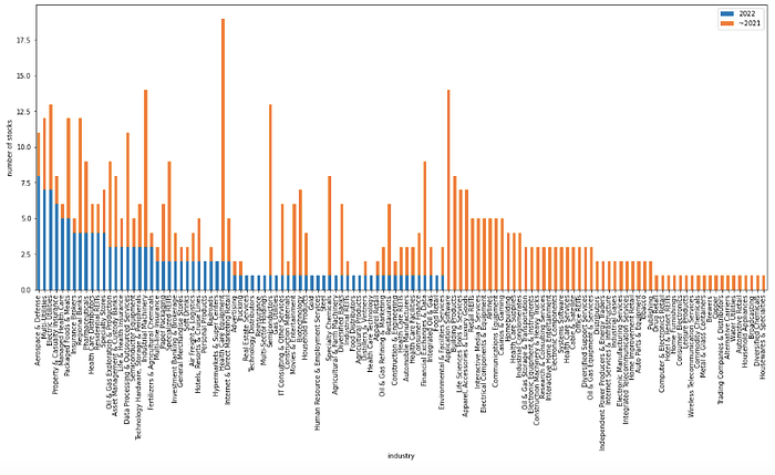
If you listen to the market, you will see that it is best to avoid industry groups that have a high percentage of stocks (in orange) that do not have the ability to make new highs. Examples include application software, building products, semiconductors, and health care equipment.
Note that we focus only on stocks in the S&P 500.
Conclusion
The stock market is rallying, but some stocks are taking the highest prices recently. It may be wiser to hold stocks that can make new highs than to hold stocks that cannot make new highs.