Introduction

The phrase "I've never seen anything more beautiful" should only be used for fractals. Sure, there is the Mona Lisa, The Starry Night, and The Birth of Venus (which all have been ruined by AI-generated art, by the way), but I don't think any artist or human could create anything royally amazing as fractals.

On the left, we have the iconic fractal, the Mandelbrot's set, discovered in 1979 when no Python or graphing software was available.

Mandelbrot's set is a set of complex numbers that, when plotted on the complex plane, forms the self-repeating shape we see. Every number in the set can also be a seed to Julia sets, and you can see the beauties appearing as I move around the mouse inside the boundary of the Mandelbrot's set.

But before we can plot the Mandelbrot or Julia sets (but, believe me, we will), we have a lot of ground to cover. If you are just here to see the cool pictures, I highly recommend downloading the open-source Fraqtive software (and go nuts!), which I used to generate the above GIF and the one below:

If you just want to plot the Mandelbrot set in Python with a single line of code, here it is (no, the subtitle was not clickbait):

from PIL import Image

Image.effect_mandelbrot((512, 512), (-3, -2.5, 2, 2.5), 100).show()

But if you want to go down the beautiful rabbit hole of fractals and learn how to plot them and, most importantly, color them appropriately, then read on!

In this post, we will learn how to plot basic (but still very cool) Mandelbrot's sets using Matplotlib and NumPy. Then, we will take things to a whole new level with Pillow in future articles.

Let's get started.

Complex numbers in Python

Python programmers don't deal with complex numbers daily. As we will work with them a lot in this tutorial, this section will serve as a primer.

You can create an imaginary part of a complex number by appending the literal j to integers or floats.

num1 = 2 + 1j
num2 = 12.3 + 23.1j

type(num1)
complex

If seeing imaginary numbers represented with j instead of i confuses you (hello, mathematicians), you can use the complex built-in function:

2 + 3j == complex(2, 3)
True

Once created, you can access the real and imaginary components of complex numbers with real and imag attributes:

num1.real
2.0
num2.imag
23.1

Another important property of complex numbers for the purposes of this article is their absolute value. An absolute value or magnitude of a complex number measures its distance from the origin (0, 0) in the complex plane. It is defined as the square root of the sum of its real and imaginary parts (thank you, Pythagoras).

abs(1 + 3.14j)
3.295390720385065

These will be enough for us to create some awesome things. Let's get started!

Simple formula, grand set

Our journey starts by finding out if some complex number c belongs to the Mandelbrot's Set, which is surprisingly easy. All we have to do is to put it through the below formula and create a sequence of z values:

The first z is always 0, as defined above. Subsequent elements are found by squaring the previous z and adding c to the result.

Let's implement the process in Python. We will define a sequence function that returns the first n elements for a given c:

def sequence(c, n=7) -> list:
    z_list = list()
    
    z = 0
    for _ in range(n):
        z = z ** 2 + c
        z_list.append(z)
    
    return z_list

Now, we will take the function on a test-drive for a bunch of numbers:

import pandas as pd

df = pd.DataFrame()
df['element'] = [f"z_{i}" for i in range(7)]

# Random numbers
cs = [0, 1, -1, 2, 0.25, -.1]

for c in cs:
    df[f"c={c}"] = sequence(c)
    
df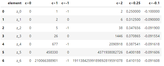

We see three types of results: when c is either 1 or 2, the sequence is unbounded (diverges to infinity) as it grows. When it is -1, it goes back and forth between 0 and -1. As for 0.25 and -0.1, they stay petite or bounded.

So, which of these five are the lucky ones to be a mandelbrot?

Are you stable?

Our screening process is stupidly simple — if c diverges the sequence to infinity, it is not in Mandelbrot's set. In fractals jargon, that c is called unstable. Or, let's ditch the negativity — the given complex number c is stable if its corresponding Z sequence remains bounded.

Now, we must figure out how many members of Z to look at before classifying c as stable or unstable. This iteration count is not obvious to find as the formula is sensitive to even the smallest changes to c.

But fortunately, people have been studying the set for a long enough time to know that all mandelbrots stay bounded within a radius of two. This means we can perform a few dozen iterations, and the numbers that remain relatively small or below 2 are probably in Mandelbrot's set.

So, let's create a new function is_stable using this logic that returns True when the number is a mandelbrot:

def is_stable(c, n_iterations=20):
    z = 0
    
    for _ in range(n_iterations):
        z = z ** 2 + c
        
        if abs(z) > 2:
            return False
    return True

In the body of this boolean function, we set z to 0 and run it through the algorithm in a loop controlled by n_iterations. In each iteration, we check the magnitude of z so that we can terminate the loop if it exceeds 2 early on and don't waste time running the rest of the iterations.

The last return statement is only executed if z is below 2 after all the iterations. Let's check a few numbers:

is_stable(1)
False
is_stable(0.2)
True
is_stable(0.26)
True
is_stable(0.26, n_iterations=30)
False

Note how increasing n_iterations to 30 changes the stability of 0.26. Generally, values close to the fractals edge require more iterations to make a more accurate classification and create more detailed visuals.

How to plot the Mandelbrot's set in Matplotlib

This section was heavily inspired by this awesome RealPython post:

Our ultimate aim for the article is to produce this guy in Matplotib (spoiler alert, we will create something even better!):

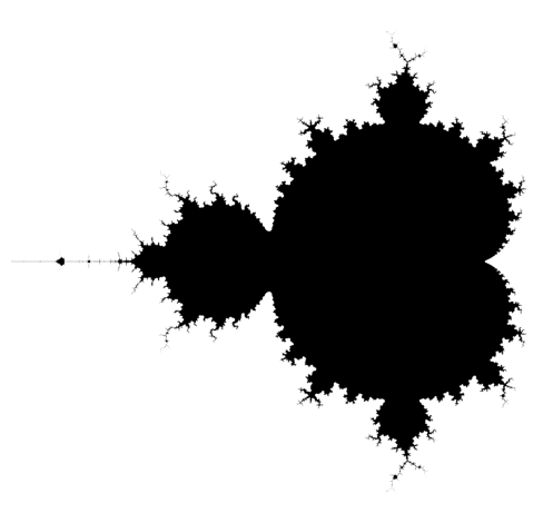
The image was created by coloring all the mandelbrots black and unstable elements white. In Matplotlib, grayscale has 256 shades or ranges from 0 to 255, 0 being fully white and 255 being pitch black. But you can normalize this range into 0 and 1 so that 0 is white and 1 is black.

This normalization comes in handy for us. We can create a 2D array of complex numbers and run our is_stable function over each element. The resulting array will have 1s for mandelbrots and 0s for the unstable. When we plot this array as an image — voila, we have the desired black-and-white visual.

Let's get to it. First, we create the function that generates a matrix of candidate values we can iterate over:

import numpy as np


def candidate_values(xmin, xmax, ymin, ymax, pixel_density):
    # Generate a 2D grid of real and imaginary values
    real = np.linspace(xmin, xmax, num=int((xmax-xmin) * pixel_density))
    imag = np.linspace(ymin, ymax, num=int((ymax-ymin) * pixel_density))
    
    # Cross each row of `xx` with each column of `yy` to create a grid of values
    xx, yy = np.meshgrid(real, imag)
    
    # Combine the real and imaginary parts into complex numbers
    matrix = xx + 1j * yy
    
    return matrix

We will use the np.linspace function to create evenly spaced numbers within a range. The pixel_density parameter dynamically sets the number of pixels per unit.

For example, a matrix with a horizontal range of (-2, 0), a vertical range of (-1.2, 1.2) and a pixel_density of 1, would have the shape (2, 2). This means our resulting Mandelbrot image would be 2 pixels wide and 2 pixels tall, which would make Benoit Mandelbrot turn in his grave.

c = candidate_values(-2, 0, -1.2, 1.2, 1)

c.shape
(2, 2)

So, we better use a higher density like 25:

c = candidate_values(-2, 0, -1.2, 1.2, 25)

c.shape
(60, 50)

Now, to run our is_stable function over each element of c, we vectorize it with np.vectorize and call it with 20 iterations:

c = candidate_values(-2, 0.7, -1.2, 1.2, pixel_density=25)

mandelbrot_mask = np.vectorize(is_stable)(c, n_iterations=20)
mandelbrot_mask.shape
(60, 67)

We are calling the resulting array a mandelbrot_mask since it returns True (1) for each mandelbrot. To plot this array, we use the imshow function of Matplpotlib with a binary colormap. That will make the image black and white.

import matplotlib.pyplot as plt

plt.imshow(mandelbrot_mask, cmap="binary")

# Turn off the axes and use tight layout
plt.axis("off")
plt.tight_layout()

Well, that is one ugly Mandelbrot. How about we increase the pixel density to 1024 and the iteration count to 30?

c = candidate_values(-2, 0.7, -1.2, 1.2, pixel_density=1024)

mandelbrot_mask = np.vectorize(is_stable)(c, n_iterations=30)

plt.imshow(mandelbrot_mask, cmap="binary")
plt.gca().set_aspect("equal")
plt.axis("off")
plt.tight_layout()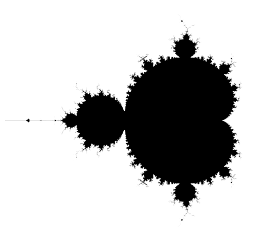

Now, this looks more like it! Congratulations on plotting your first Mandelbrot image!

Wait, that wasn't art!

Even though our current fractal still looks very cool, it is far from the art I promised.

So, let's give it a makeover by focusing on not just the black set numbers but on the numbers around the edge. Because looking at this image, we can see all types of interesting patterns emerging around the boundaries:

Let's start the makeover by organizing our code into a class because it is a real mess with everything scattered.

The class name will be Mandelbrot and we will use data classes so that we don't have to create the __init__ constructor like a caveman:

from dataclasses import dataclass

@dataclass
class Mandelbrot: # Inspired by the Real Python article shared above
    n_iterations: int
    
    def is_stable(self, c: complex) -> bool:
        z = 0
    
        for _ in range(self.n_iterations):
            z = z ** 2 + c
            if abs(z) > 2:
                return False

        return True

The class only requires the max_iteration parameter to be initialized. We also add the is_stable function as a class method.

mandelbrot = Mandelbrot(n_iterations=30)

mandelbrot.is_stable(0.1)
True
mandelbrot.is_stable(1 + 4.4j)
False

Up until now, we have been coloring only the mandelbrots black and the rest white. But if we want to spice up the edges of the set, we have to come up with a logic to color the unstable elements other than white.

One way we can do this is by determining in how many iterations a complex number becomes unstable. Some will become unstable very fast (maybe they have short fuses?), but others may take hundreds or thousands of iterations (they are patient). In general, though, numbers close to the fractal's edge are less unstable (take more iterations) than those far away.

Using this information, we can give each pixel (complex number) different depths of color based on the iteration they terminate. This is called the Escape Count algorithm. Let's implement it in our class:

@dataclass
class Mandelbrot:
    max_iterations: int
    
    def escape_count(self, c: complex) -> int:
        z = 0
        for iteration in range(self.max_iterations):
            z = z ** 2 + c
            if abs(z) > 2:
                return iteration
        return self.max_iterations

First, we change n_iterations to max_iterations, as it makes more sense. Then, we create an escape_count method that:

• if c is unstable, returns the iteration in which it exceeds the magnitude of 2
• if c is stable, returns the max iteration count

mandelbrot = Mandelbrot(max_iterations=50)

mandelbrot.escape_count(-0.1) # stable
50
mandelbrot.escape_count(0.26) # unstable
29

Now, we create another method to measure the stability based on the iteration count:

@dataclass
class Mandelbrot:
    max_iterations: int
    
    def escape_count(self, c: complex) -> int:
        z = 0
        for i in range(self.max_iterations):
            z = z ** 2 + c
            if abs(z) > 2:
                return i
        return self.max_iterations
    
    def stability(self, c: complex) -> float:
        return self.escape_count(c) / self.max_iterations

The stability method returns a measure between 0 and 1, which we can later use to determine the color depths. Only mandelbrots will return max_iterations, so they will be marked with 1. Numbers close to the edge will take longer to become unstable, so they will have increasingly closer values to 1.

With this logic, we can bring back our is_stable function but make it much shorter:

@dataclass
class Mandelbrot:
    max_iterations: int
    
    def escape_count(self, c: complex) -> int:
        z = 0
        for i in range(self.max_iterations):
            z = z ** 2 + c
            if abs(z) > 2:
                return i
        return self.max_iterations
    
    def stability(self, c: complex) -> float:
        return self.escape_count(c) / self.max_iterations
    
    def is_stable(self, c: complex) -> bool:
        # Return True only when stability is 1
        return self.stability(c) == 1
mandelbrot = Mandelbrot(max_iterations=50)

mandelbrot.stability(-.1)
1.0
mandelbrot.is_stable(-.1)
True
mandelbrot.stability(2)
0.02
mandelbrot.is_stable(2)
False

Now, we create a final method to plot the set with Matplotlib:

@dataclass
class Mandelbrot:
    max_iterations: int
    
    # ... The rest of the code from above
    
    @staticmethod
    def candidate_values(xmin, xmax, ymin, ymax, pixel_density):
        real = np.linspace(xmin, xmax, num=int((xmax-xmin) * pixel_density))
        imag = np.linspace(ymin, ymax, num=int((ymax-ymin) * pixel_density))

        xx, yy = np.meshgrid(real, imag)
        matrix = xx + 1j * yy

        return matrix
    
    
    def plot(self, xmin, xmax, ymin, ymax, pixel_density=64, cmap="gray_r"):
        c = Mandelbrot.candidate_values(xmin, xmax, ymin, ymax, pixel_density)
        
        # Apply `stability` over all elements of `c`
        c = np.vectorize(self.stability)(c)
        
        plt.imshow(c, cmap=cmap, extent=[0, 1, 0, 1])
        plt.gca().set_aspect("equal")
        plt.axis('off')
        plt.tight_layout()

In plot, we apply the stability method over all elements of c, so the resulting matrix holds color depths in each cell. When we plot this matrix with a reversed grayscale colormap (so that the mandelbrots stay black), we get the following image:

mandelbrot = Mandelbrot(max_iterations=30)

mandelbrot.plot(
    xmin=-2, xmax=0.5, 
    ymin=-1.5, ymax=1.5, 
    pixel_density=1024,
)

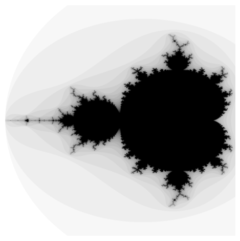
We can already see bands with different levels of grey appearing around the edges. Let's give it another colormap that isn't boring grayscale:

mandelbrot = Mandelbrot(max_iterations=30)

mandelbrot.plot(
    xmin=-2, xmax=0.5, 
    ymin=-1.5, ymax=1.5, 
    pixel_density=1024,
    cmap="gist_heat"
)

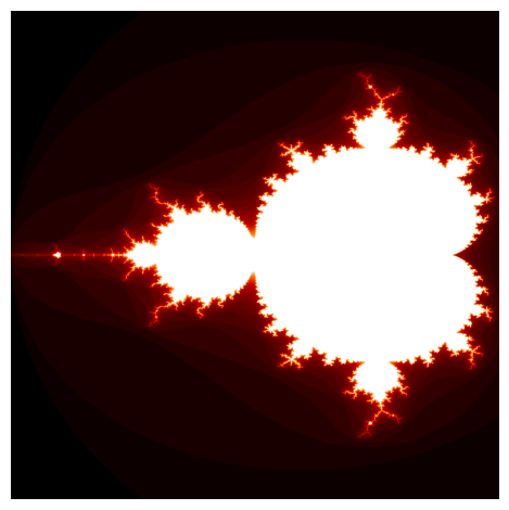
Pay attention to how the boundary lines are the brightest red and how white spots still appear where the set repeats itself. Awesome!

Conclusion

Our final result was almost art. But, there are a lot of improvements we can make. The first thing is improving the image resolution by having finer control over each pixel. Then, we have to remove that annoying white space around the image (if you are reading in dark mode).

All these tasks are shortcomings of Matplotlib, but in the next article, we will take things to a whole new level with Pillow, Python's image manipulation library.

Stay tuned!

Loved this article and, let's face it, its bizarre writing style? Imagine having access to dozens more just like it, all written by a brilliant, charming, witty author (that's me, by the way :).

For only 4.99$ membership, you will get access to not just my stories, but a treasure trove of knowledge from the best and brightest minds on Medium. And if you use my referral link, you will earn my supernova of gratitude and a virtual high-five for supporting my work.