This article has 2 parts: 1. Theory behind conditional probability 2. Example with python
Part 1: Theory and formula behind conditional probability
For once, wikipedia has an approachable definition,
In probability theory, conditional probability is a measure of the probability of an event occurring given that another event has (by assumption, presumption, assertion or evidence) occurred.
Translation: given B is true, what is the probability that A is also true.
It's easier to understand something with concrete examples. Below are a few random examples of conditional probabilities we could calculate.
Examples:
- What's the probability of someone sleeping less than 8 hours if they're a college student.
- What's the probability of a dog living longer than 15 years if they're a border collie.
- What's the probability of using all your vacation days if you work for the government.
Formula:

The formula for conditional probability is P(A|B) = P(A ∩ B) / P(B).
The parts: P(A|B) = probability of A occurring, given B occurs P(A ∩ B) = probability of both A and B occurring P(B) = probability of B occurring
| means "given". Meaning "in cases where something else occurs".
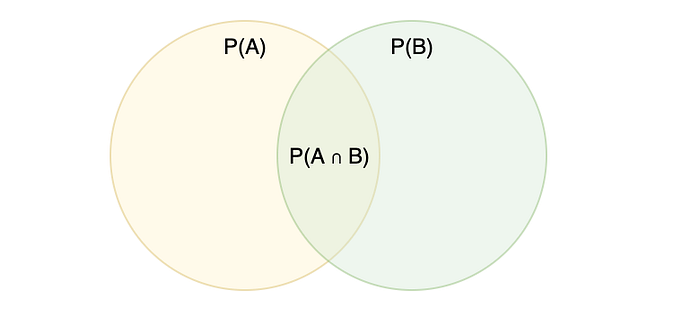
∩ means intersection which you can think of as and, or the overlap in the context of a Venn diagram.

But why do we divide P(A ∩ B) by P(B)in the formula?
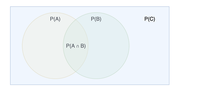
Because we want to exclude the probability of non-B cases. We're scoping our probability to that falling within B.

Dividing byP(B) removes the probability of anything not B . C — B above.
Part 2: Example with python
We're going to calculate the probability a student gets an A (80%+) in math, given they miss 10 or more classes.
Download the dataset from kaggle and inspect the data.
import pandas as pd
df = pd.read_csv('student-alcohol-consumption/student-mat.csv')
df.head(3)
And check the number of records.
len(df)
#=> 395
We're only concerned with the columns, absences (number of absences), and G3 (final grade from 0 to 20).
Let's create a couple new boolean columns based on these columns to make our lives easier.
Add a boolean column called grade_A noting if a student achieved 80% or higher as a final score. Original values are on a 0–20 scale so we multiply by 5.
df['grade_A'] = np.where(df['G3']*5 >= 80, 1, 0)Make another boolean column called high_absenses with a value of 1 if a student missed 10 or more classes.
df['high_absenses'] = np.where(df['absences'] >= 10, 1, 0)Add one more column to make building a pivot table easier.
df['count'] = 1And drop all columns we don't care about.
df = df[['grade_A','high_absenses','count']]
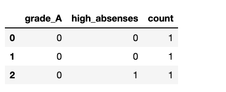
df.head()
Nice. Now we'll create a pivot table from this.
pd.pivot_table(
    df,
    values='count',
    index=['grade_A'],
    columns=['high_absenses'],
    aggfunc=np.size,
    fill_value=0
)
We now have all the data we need to do our calculation. Let's start by calculating each individual part in the formula.
In our case:
P(A) is the probability of a grade of 80% or greater.
P(B) is the probability of missing 10 or more classes.
P(A|B) is the probability of a 80%+ grade, given missing 10 or more classes.
Calculations of parts: P(A) = (35 + 5) / (35 + 5 + 277 + 78) = 0.10126582278481013 P(B) = (78 + 5) / (35 + 5 + 277 + 78) = 0.21012658227848102 P(A ∩ B) = 5 / (35 + 5 + 277 + 78) = 0.012658227848101266
And per the formula, P(A|B) = P(A ∩ B) / P(B), put it together.
P(A|B) = 0.012658227848101266/ 0.21012658227848102= 0.06
There we have it. The probability of getting at least an 80% final grade, given missing 10 or more classes is 6%.
Conclusion
While the learning from our specific example is clear - go to class if you want good grades, conditional probability can be applied to more serious circumstances.
For example, the probability a person has a particular disease, given test results.
An understanding is also essential before diving into more complicated probability estimations using Bayes' theorem.

