Along the way, we'll address challenges and techniques specific to large-scale model development, including:

• Collecting and preparing massive datasets for training
• Building a custom tokenizer tailored to the domain and corpus
• Scaling training across multiple GPUs to handle billions of parameters

To make this possible, we'll leverage PyTorch's Accelerate library — a powerful tool designed to simplify distributed training and optimize large-scale workflows. While the Hugging Face Trainer supports multi-GPU setups, Accelerate offers more flexibility and performance for custom training loops.

Large Datasets and Where to Find Them

In domains like law, biomedicine, or software engineering, it's common to have access to vast amounts of data. However, this data is often unlabeled, and labeling at scale can be prohibitively expensive or time-consuming. Still, such datasets can play a crucial role in improving model performance, particularly through domain adaptation techniques. Even when labels are absent or heuristically derived, these corpora offer unique opportunities to fine-tune or pretrain language models more effectively.

Key takeaways include:

1.Heuristics and metadata are often the only viable methods for labeling large datasets at scale.

2.Fine-tuning on unlabeled domain-specific data can significantly boost model performance when labeled data is limited.

3.The decision to fine-tune vs. train from scratch depends on:

• The extent of the domain gap between your data and existing pretrained models.

4.Relying on a pretrained tokenizer (e.g., from GPT) can lead to poor results when working with specialized domains such as legal texts, code, or biological sequences.

5.When your dataset approaches the size of those used in large-scale pretraining, and computational resources allow, training both the model and tokenizer from scratch becomes a compelling option.

Before diving into specific pretraining objectives, it's essential to first construct a large, well-curated corpus that reflects the nuances of your target domain.

"Pretraining Language Models for Biomedical NLP (BioBERT PDF)"

Challenges of Building a Large-Scale Pretraining Corpus

The performance and behavior of a Transformer model after pretraining are deeply tied to the quality of its training corpus. Any flaws, imbalances, or biases present in the dataset are likely to be inherited by the model itself. As a result, constructing a large corpus for pretraining is not just a matter of collecting massive amounts of text — it's a nuanced process that requires thoughtful curation and an awareness of potential risks.

As datasets scale up, controlling their contents becomes increasingly difficult. Unlike carefully curated datasets crafted by domain experts, most large-scale corpora are compiled automatically or semi-automatically, often using data generated as a byproduct of other processes — like web scraping, document archiving, or logging user behavior. This introduces several important challenges:

Key Issues in Large-Scale Corpus Construction

1.Lack of Content Control: With large, automated datasets, it's hard to maintain precise oversight of what's included, increasing the risk of irrelevant, biased, or low-quality data.

2.Bias and Representation Gaps: Studies of large corpora like C4 (used for T5) and BookCorpus (used for BERT) have revealed:

• A large portion of C4 includes machine-translated text rather than professionally translated content.
• African-American English is underrepresented due to over-aggressive stopword filtering.
• Words related to gender and sexuality — even common, non-explicit ones like "sex" — are sometimes entirely missing due to content filtering.
• Content Skew: BookCorpus, for example, contains a disproportionate amount of romance novels, skewing the model's learned representations toward that genre.
• Copyright Concerns: Both C4 and BookCorpus have been found to include copyrighted content, raising legal and ethical questions around data usage.

Despite these issues, such datasets are still widely used. In some cases, these biases or content skews may be acceptable — for example, if you're building a model specifically designed for generating romance novels or interactive storytelling games.

References & Further Reading:

• Datasheet for BookCorpus (Bandy & Vincent, 2021)
• Documenting the English Colossal Clean Crawled Corpus (Dodge et al., 2021)

Let's illustrate the notion of a model being skewed by the data by comparing text gen‐ erations from GPT and GPT-2. GPT was mostly trained on BookCorpus, while GPT-2 was trained on web pages, blogs, and news articles linked from Reddit. We'll compare similar-sized versions of both models on the same prompt, so that the main difference is the pretraining dataset, and we'll use the text-generation pipeline to investigate the model outputs:

from transformers import pipeline, set_seed
generation_gpt = pipeline("text-generation", model="openai-gpt")
generation_gpt2 = pipeline("text-generation", model="gpt2")

Next, let's create a simple function to count the number of parameters in each model:

def model_size(model):
 return sum(t.numel() for t in model.parameters())
print(f"GPT size: {model_size(generation_gpt.model)/1000**2:.1f}M parameters")
print(f"GPT2 size: {model_size(generation_gpt2.model)/1000**2:.1f}M parameters")

Output:

GPT size: 116.5M parameters
GPT2 size: 124.4M parameters

The original GPT model is about the same size as the smallest GPT-2 model. Now we can generate three different completions from each model, each with the same input prompt:

ef enum_pipeline_ouputs(pipe, prompt, num_return_sequences):
 out = pipe(prompt, num_return_sequences=num_return_sequences,
 clean_up_tokenization_spaces=True)
 return "\n".join(f"{i+1}." + s["generated_text"] for i, s in enumerate(out))
prompt = "\nWhen they came back"
print("GPT completions:\n" + enum_pipeline_ouputs(generation_gpt, prompt, 3))
print("")
print("GPT-2 completions:\n" + enum_pipeline_ouputs(generation_gpt2, prompt, 3))

Output:

GPT completions:
1.
When they came back.
 " we need all we can get, " jason said once they had settled into the back of
the truck without anyone stopping them. " after getting out here, it 'll be up
to us what to find. for now
2.
When they came back.
 his gaze swept over her body. he 'd dressed her, too, in the borrowed clothes
that she 'd worn for the journey.
 " i thought it would be easier to just leave you there. " a woman like
3.
When they came back to the house and she was sitting there with the little boy
 " don't be afraid, " he told her. she nodded slowly, her eyes wide. she was so
lost in whatever she discovered that tom knew her mistake
GPT-2 completions:
1.
When they came back we had a big dinner and the other guys went to see what
their opinion was on her. I did an hour and they were happy with it.
2.
When they came back to this island there had been another massacre, but he could
not help but feel pity for the helpless victim who had been left to die, and
that they had failed that day. And so was very, very grateful indeed.
3.
When they came back to our house after the morning, I asked if she was sure. She
said, "Nope." The two kids were gone that morning. I thought they were back to
being a good friend.

In general, any model trained on a dataset will reflect the language bias and over- or underrepresentation of populations and events in its training data. These biases in the behavior of the model are important to take into consideration with regard to the tar‐ get audience interacting with the model; for some useful guidelines, we refer you to a paper by Google that provides a framework for dataset development.

Building a Custom Code Dataset

To narrow the scope and simplify the challenge of training from scratch, let's focus on building a code generation model for Python. The first requirement is a large, high-quality corpus of Python source code — and thankfully, one of the world's richest resources for this already exists: GitHub.

GitHub hosts over 20 million code repositories, containing everything from small test projects to large production-grade applications. With careful filtering and licensing awareness, GitHub becomes an invaluable source for pretraining a Transformer model on real-world code.

Why GitHub?

• GitHub repositories are widely used, well-documented, and cover diverse coding styles and libraries.
• Much of the content is open source and freely accessible, subject to license constraints.
• Projects include everything from beginner-level scripts to full-scale frameworks — ideal for capturing the full range of Python syntax and structure.

How to Access GitHub Data for Pretraining

There are two main ways to retrieve code from GitHub:

• GitHub REST API: Useful for smaller-scale tasks (e.g., downloading issues or metadata), but limited by rate constraints.
• Google BigQuery Public Datasets: The preferred method for large-scale extraction Specifically:

1.Use the bigquery-public-data.github_repos.contents table.

2.This table includes all ASCII files under 10MB from public, open-source repositories.

3.File inclusion is based on licenses as identified by the GitHub License API.

📌 Tip: Make sure to filter files by language and content type to avoid non-code files (e.g., README.md, LICENSE, etc.).

📄 Reference:

• Unsupervised Translation of Programming Languages (Lachaux et al 2020)

Creating a dataset with Google BigQuery

1. Create a Google Cloud account (a free trial should be sufficient).
2. Create a Google BigQuery project under your account.
3. In this project, create a dataset.
4. In this dataset, create a table where the results of the SQL request will be stored.
5. Prepare and run the following SQL query on the github_repos (to save the query results, select More > Query Options, check the "Set a destination table for query results" box, and specify the table name):

SELECT
 f.repo_name, f.path, c.copies, c.size, c.content, l.license
FROM
 `bigquery-public-data.github_repos.files` AS f
JOIN
 `bigquery-public-data.github_repos.contents` AS c
ON
 f.id = c.id
JOIN
 `bigquery-public-data.github_repos.licenses` AS l
ON
 f.repo_name = l.repo_name
WHERE
 NOT c.binary
 AND ((f.path LIKE '%.py')
 AND (c.size BETWEEN 1024
 AND 1048575))

After running the BigQuery extraction, the process yields around 26.8 million Python files — amounting to 2.6 TB of raw data, which is then compressed into a manageable 50 GB of JSON files. Each file contains usable Python source code suitable for pretraining a code generation model.

To ensure quality and efficiency, the dataset is carefully filtered:

• Empty and trivial files (like __init__.py) are removed.
• Large files exceeding 1 MB are excluded to reduce outlier noise.
• Licenses are downloaded for all files to allow license-based filtering later.

Requirements Before Downloading

• A stable, high-speed internet connection
• Minimum 50 GB of free local disk space
• A Google Cloud account with access to Google Cloud Storage (GCS)

Next, we'll download the results to our local machine.

Export your results to Google Cloud:

• Create a bucket and a folder in Google Cloud Storage (GCS).
• Export your table to this bucket by selecting Export > Export to GCS, with an export format of JSON and gzip compression.

To download the bucket to your machine, use the gsutil library:

• Install gsutil with pip install gsutil.
• Configure gsutil with your Google account: gsutil config.
• Copy your bucket on your machine:

$ gsutil -m -o "GSUtil:parallel_process_count=1" cp -r gs://

Alternatively, you can directly download the dataset from the Hugging Face Hub with the following command:

Working with Large Datasets

Loading and managing large datasets is a common challenge in machine learning, especially when the dataset size exceeds the available system RAM. For large-scale pretraining tasks, this is almost inevitable. In our example, we're working with 50 GB of compressed data, which expands to approximately 200 GB once uncompressed — a scale that quickly outpaces the capabilities of standard laptops and desktops.

Fortunately, the 🤗 datasets library is built to handle these limitations efficiently with two key features:

• Memory mapping
• Streaming

Loading a Large Local Dataset

from datasets import load_dataset, DownloadConfig

download_config = DownloadConfig(delete_extracted=True)
dataset = load_dataset("./codeparrot", split="train", download_config=download_config)

This approach:

• Decompresses your JSON files (requires ~180 GB disk space)
• Automatically deletes extracted files after caching to save space

Check Size and Memory Usage

import os, psutil

print(f"Number of Python files in dataset: {len(dataset)}")

ds_size = sum(os.stat(f["filename"]).st_size for f in dataset.cache_files)
print(f"Dataset size (cache file): {ds_size / 2**30:.2f} GB")

ram_used = psutil.Process(os.getpid()).memory_info().rss >> 20
print(f"RAM used: {ram_used} MB")

Output:

Number of Python files in dataset: 18,695,559  
Dataset size (cache file): 183.68 GB  
RAM used: 4924 MB

Streaming

When even disk space becomes a constraint, you can stream the dataset instead of storing it locally. The streaming mode reads the data on-the-fly without caching or decompressing the entire dataset.

Streaming supports formats such as:

• JSON Lines
• CSV
• Text (raw or compressed: .zip, .gz, .zst)

streamed_dataset = load_dataset('./codeparrot', split="train", streaming=True)

• The dataset is loaded instantly
• It behaves as an IterableDataset, meaning no random access (e.g., dataset[100])
• Use next(iter(dataset)) to access samples sequentially

You can still shuffle the data:

streamed_dataset = streamed_dataset.shuffle(buffer_size=1000)

This fetches a buffer of 1,000 examples at a time and shuffles within it.

Verifying Sample Consistency

iterator = iter(streamed_dataset)
print(dataset[0] == next(iterator))  # True
print(dataset[1] == next(iterator))  # True

Even in streaming mode, the dataset provides identical results to the memory-mapped version.

Streaming Directly from the Hub

To minimize both RAM and disk usage, you can stream datasets directly from the Hugging Face Hub — no downloads or decompression required.

remote_dataset = load_dataset('transformersbook/codeparrot', split="train", streaming=True)

This lets you work with arbitrarily large datasets on a tiny machine, ideal for cost-effective cloud training or quick experimentation.

By combining memory mapping and streaming, Hugging Face datasets allows you to scale your training workflows far beyond your machine's physical constraints—with almost no trade-offs in usability or performance.

Adding Datasets to the Hugging Face Hub

Once you've built and prepared your dataset, a great way to manage, share, and access it efficiently is by uploading it to the Hugging Face Hub. Doing so provides several benefits:

• 🔄 Seamless access from your training servers or notebooks
• 🌐 Effortless dataset streaming using the datasets library
• 🤝 Community sharing, so others can explore or contribute

Before uploading anything, log in to your Hugging Face account via the CLI:

huggingface-cli login

Alternatively, use notebook_login() if you're working in a notebook environment.

huggingface-cli repo create --type dataset --organization transformersbook codeparrot-train
huggingface-cli repo create --type dataset --organization transformersbook codeparrot-valid

If you're uploading under your personal account, omit the --organization flag.

Download the empty dataset repositories to your local machine:

git clone https://huggingface.co/datasets/transformersbook/codeparrot-train
git clone https://huggingface.co/datasets/transformersbook/codeparrot-valid

Upload Training Files

cd codeparrot-train
cp ../codeparrot/*.json.gz .
rm ./file-000000000183.json.gz  # Reserve the last file for validation
git add .
git commit -m "Adding dataset files"
git push

Upload Validation File

cd ../codeparrot-valid
cp ../codeparrot/file-000000000183.json.gz .
mv ./file-000000000183.json.gz ./file-000000000183_validation.json.gz
git add .
git commit -m "Adding dataset files"
git push

🕐 Note: git add . may take some time since hashes are computed for each file. Upload time will also vary depending on file size and network speed.

And that's it! Our two splits of the dataset as well as the full dataset are now live on the Hugging Face Hub at the following URLs:

• https://huggingface.co/datasets/transformersbook/codeparrot

• https://huggingface.co/datasets/transformersbook/codeparrot-train

• https://huggingface.co/datasets/transformersbook/codeparrot-valid

Building a Tokenizer

However, when we train a new model, using a tokenizer prepared for another dataset can be suboptimal. Here are a few examples of the kinds of problems we might run into when using an existing tokenizer:

• The T5 tokenizer was trained on the C4 corpus that we encountered earlier, but an extensive step of stopword filtering was used to create it. As a result, the T5 tokenizer has never seen common English words such as "sex."
• The CamemBERT tokenizer was also trained on a very large corpus of text, but only comprising French text (the French subset of the OSCAR corpus). As such, it is unaware of common English words such "being."

We can easily test these features of each tokenizer in practice:

from transformers import AutoTokenizer
def tok_list(tokenizer, string):
 input_ids = tokenizer(string, add_special_tokens=False)["input_ids"]
 return [tokenizer.decode(tok) for tok in input_ids]
tokenizer_T5 = AutoTokenizer.from_pretrained("t5-base")
tokenizer_camembert = AutoTokenizer.from_pretrained("camembert-base")
print(f'T5 tokens for "sex": {tok_list(tokenizer_T5,"sex")}')
print(f'CamemBERT tokens for "being": {tok_list(tokenizer_camembert,"being")}')

Output:

T5 tokens for "sex": ['', 's', 'ex']
CamemBERT tokens for "being": ['be', 'ing']

The Tokenizer Model

we learned that a tokenizer is a processing pipeline consisting of four key stages:

• Normalization
• Pretokenization
• Tokenizer model (trainable
• Postprocessing

Among these, only the tokenizer model itself is trainable, and its performance depends significantly on the algorithm used. Here are the main subword tokenization algorithms commonly applied in NLP:

🔤 Byte Pair Encoding (BPE)

• Begins with a vocabulary of single characters as the base units.
• Iteratively merges the most frequent pairs of tokens to form new tokens.
• This merging continues until the tokenizer reaches a predefined vocabulary size.
• Known for being simple and effective, and widely adopted in models like GPT and RoBERTa.

🧩 Unigram Language Model

• Starts from the entire corpus vocabulary, including all words and possible subwords.
• Then progressively removes or splits tokens that contribute least to performance.
• Continues pruning until the target vocabulary size is reached.
• Often performs better with diverse text types due to its probabilistic nature.

🧬 WordPiece

• Conceptually a predecessor to Unigram, used in models like BERT.
• Focuses on maximizing the likelihood of the training data using a fixed vocabulary.
• The official implementation by Google was never open-sourced, but alternatives exist.

⚖️ Comparative Insights

• No single algorithm is universally superior; performance depends on the dataset and downstream task.
• BPE and Unigram generally offer strong and consistent results across many scenarios.

Key evaluation criteria include:

• Token efficiency (fewer tokens per sentence)
• Handling of rare or domain-specific words
• Vocabulary adaptability and size

Measuring Tokenizer Performance

Evaluating the effectiveness of a tokenizer isn't straightforward. While various metrics can provide valuable insights, they each offer a partial view of overall performance. Below are some key measures commonly used to assess tokenizer quality:

📊 Common Evaluation Metrics

1.Subword Fertility Measures the average number of subwords per tokenized word. → Lower fertility typically means more compact tokenization.

2.Proportion of Continued Words Indicates the percentage of words split into multiple subtokens. → High values may suggest over-fragmentation of the text.

3.Coverage Metrics Evaluate how well the tokenizer handles vocabulary coverage. Examples:

• Proportion of unknown (OOV) tokens
• Usage frequency of rare tokens

4.Robustness to Noise and Misspellings Assesses the tokenizer's ability to handle out-of-domain inputs such as typos or inconsistent formatting.

🤖 Tokenizer–Model Interaction

Although these metrics offer useful diagnostic signals, they do not capture the interaction between the tokenizer and the model. For instance:

• A tokenizer with minimal subword fertility might simply include most full words in its vocabulary.
• While this seems efficient, it can lead to huge vocabulary sizes, making the model harder to train and generalize.

🧪 Downstream Task Performance

Ultimately, the most reliable way to evaluate a tokenizer is through the performance of the model trained with it. For example:

• Early success of BPE (Byte Pair Encoding) was demonstrated by significant gains in machine translation tasks, when compared to traditional word- or character-based tokenization.

A Tokenizer for Python

We need a custom tokenizer for our use case: tokenizing Python code. The question of pretokenization merits some discussion for programming languages.

Let's see if there are any tokenizers in the collection provided on the Hub that might be useful to us.Let's load this tokenizer and explore its tokenization properties:

from transformers import AutoTokenizer
python_code = r"""def say_hello():
 print("Hello, World!")
# Print it
say_hello()
"""
tokenizer = AutoTokenizer.from_pretrained("gpt2")
print(tokenizer(python_code).tokens())

Output:

['def', 'Ġsay', '_', 'hello', '():', 'Ċ', 'Ġ', 'Ġ', 'Ġ', 'Ġprint', '("',
'Hello', ',', 'ĠWorld', '!"', ')', 'Ġ#', 'ĠPrint', 'Ġit', 'Ċ', 'Ċ', 'say', '_',
'hello', '()', 'Ċ']

This output seems rather unusual, so let's break it down by examining each component of the tokenizer pipeline. To start, we'll inspect the normalization step to understand what transformations are being applied.

print(tokenizer.backend_tokenizer.normalizer)
None

As we can see, the GPT-2 tokenizer uses no normalization. It works directly on the raw Unicode inputs without any normalization steps. Let's now take a look at the pretokenization:

print(tokenizer.backend_tokenizer.pre_tokenizer.pre_tokenize_str(python_code))

Output :

[('def', (0, 3)), ('Ġsay', (3, 7)), ('_', (7, 8)), ('hello', (8, 13)), ('():',
(13, 16)), ('ĊĠĠĠ', (16, 20)), ('Ġprint', (20, 26)), ('("', (26, 28)), ('Hello',
(28, 33)), (',', (33, 34)), ('ĠWorld', (34, 40)), ('!")', (40, 43)), ('Ġ#', (43,
45)), ('ĠPrint', (45, 51)), ('Ġit', (51, 54)), ('Ċ', (54, 55)), ('Ċ', (55, 56)),
('say', (56, 59)), ('_', (59, 60)), ('hello', (60, 65)), ('()', (65, 67)), ('Ċ',
(67, 68))]

Let's begin by examining the numbers. One powerful feature of tokenizers is offset tracking, which allows us to map tokens back to their exact positions in the original text. This means every transformation applied to the input string is recorded, so after tokenization, we can still trace each token back to its original character span. For instance, the word "hello" might correspond to characters 8 through 13 in the original input. Even when normalization removes certain characters, this tracking maintains the link between the original and processed text.

You may have also noticed some unusual-looking tokens, such as Ċ and Ġ. These stem from byte-level tokenization, where the model operates on raw bytes rather than Unicode characters. Since Unicode characters can span from one to four bytes, this approach normalizes the input to a compact 256-element byte alphabet—making it possible to represent any Unicode string using just byte combinations.

Why use bytes at all? While the Unicode alphabet contains over 143,000 characters, the byte alphabet is fixed at 256, allowing us to tokenize any string — no matter the language — using a consistent base. For example:

a, e = u"a", u"€"
print(f"`{a}`: {a.encode('utf-8')} → byte: {ord(a.encode('utf-8'))}")
print(f"`{e}`: {e.encode('utf-8')} → bytes: {[ord(chr(i)) for i in e.encode('utf-8')]}")

Output:

`a`: b'a' → byte: 97
`€`: b'\xe2\x82\xac' → bytes: [226, 130, 172]

Using only bytes, however, results in longer sequences, as each Unicode character is split into multiple bytes. This adds computation overhead for the model, especially when reconstructing meaningful tokens. As a solution, algorithms like Byte Pair Encoding (BPE) offer a compromise: they start with a basic vocabulary (like bytes) and iteratively merge frequently co-occurring tokens (e.g., t and h → th), expanding the vocabulary to better reflect language patterns.

It's worth noting that the "byte" in BPE refers to a legacy compression technique, not literal bytes as in byte-level tokenization. In NLP, BPE typically works with Unicode strings. To bridge this, tokenizers like GPT-2's map the 256 byte values to unique, printable Unicode characters — ensuring compatibility with character-based BPE algorithms.

You can view this byte-to-Unicode mapping using:

from transformers.models.gpt2.tokenization_gpt2 import bytes_to_unicode
byte_to_unicode_map = bytes_to_unicode()
unicode_to_byte_map = dict((v, k) for k, v in byte_to_unicode_map.items())
base_vocab = list(unicode_to_byte_map.keys())
print(f'Size of our base vocabulary: {len(base_vocab)}')
print(f'First element: `{base_vocab[0]}`, last element: `{base_vocab[-1]}`')

#OUTPUT
Size of our base vocabulary: 256
First element: `!`, last element: `Ń`

This returns a base vocabulary of 256 printable characters, including mappings like:

• Space ( ) → Ġ
• Newline (\n) → Ċ
• Carriage return → č

Running GPT-2's tokenizer on Python code illustrates this mapping. Spaces become Ġ, newlines become Ċ, and multi-space indentation appears as repeated Ġ tokens. However, because the tokenizer wasn't trained specifically on code (where indentation matters), it treats these as ordinary sequences. This limits its ability to efficiently tokenize code structures.

The final GPT-2 tokenizer vocabulary consists of 50,257 tokens:

• 256 byte-level tokens
• 50,000 BPE-learned tokens
• 1 special document boundary token

You can check this using

print(f"Tokenizer vocab size: {len(tokenizer)}")

Applying this tokenizer to code will yield a sequence of tokens that preserve words but split longer whitespace segments. This is a clear case of domain mismatch. To improve results, especially for structured inputs like code, we need to train a tokenizer specifically on code samples — something we'll explore next.

Training a Tokenizer

Let's retrain our byte-level BPE tokenizer on a slice of our corpus to get a vocabulary better adapted to Python code. Retraining a tokenizer provided by Transformers is simple. We just need to:

• Specify our target vocabulary size.
• Prepare an iterator to supply lists of input strings to process to train the tokeniz‐ er's model.
• Call the train_new_from_iterator() method.

tokens = sorted(tokenizer.vocab.items(), key=lambda x: len(x[0]), reverse=True)
print([f'{tokenizer.convert_tokens_to_string(t)}' for t, _ in tokens[:8]]);

Now let's have a look at the last words that were added to the vocabulary, and thus the least frequent ones:

tokens = sorted(tokenizer.vocab.items(), key=lambda x: x[1], reverse=True)
print([f'{tokenizer.convert_tokens_to_string(t)}' for t, _ in tokens[:12]]);
['<|endoftext|>', ' gazed', ' informants', ' Collider', ' regress', 'ominated',
' amplification', 'Compar', '..."', ' (/', 'Commission', ' Hitman']

Let's train a fresh tokenizer on our corpus and examine its learned vocabulary. Since we just need a corpus reasonably representative of our dataset statistics, let's select about 1–2 GB of data, or about 100,000 documents from our corpus:

from tqdm.auto import tqdm
length = 100000
dataset_name = 'transformersbook/codeparrot-train'
dataset = load_dataset(dataset_name, split="train", streaming=True)
iter_dataset = iter(dataset)
def batch_iterator(batch_size=10):
 for _ in tqdm(range(0, length, batch_size)):
 yield [next(iter_dataset)['content'] for _ in range(batch_size)]
new_tokenizer = tokenizer.train_new_from_iterator(batch_iterator(),
 vocab_size=12500,
initial_alphabet=base_vocab)

Let's investigate the first and last words created by our BPE algorithm to see how rele‐ vant our vocabulary is. We skip the 256 byte tokens and look at the first tokens added thereafter:

tokens = sorted(new_tokenizer.vocab.items(), key=lambda x: x[1], reverse=False)
print([f'{tokenizer.convert_tokens_to_string(t)}' for t, _ in tokens[257:280]]);


[' ', ' ', ' ', ' ', 'se', 'in', ' ', 're', 'on', 'te', '\n
', '\n ', 'or', 'st', 'de', '\n ', 'th', 'le', ' =', 'lf', 'self',
'me', 'al']

Now let's check out the last words:

print([f'{new_tokenizer.convert_tokens_to_string(t)}' for t,_ in tokens[-12:]]);


[' capt', ' embedded', ' regarding', 'Bundle', '355', ' recv', ' dmp', ' vault',
' Mongo', ' possibly', 'implementation', 'Matches']

We can also tokenize our simple example of Python code to see how our tokenizer is behaving on a simple example:

print(new_tokenizer(python_code).tokens())

['def', 'Ġs', 'ay', '_', 'hello', '():', 'ĊĠĠĠ', 'Ġprint', '("', 'Hello', ',',
'ĠWor', 'ld', '!")', 'Ġ#', 'ĠPrint', 'Ġit', 'Ċ', 'Ċ', 's', 'ay', '_', 'hello',
'()', 'Ċ']

Let's check if all the Python reserved keywords are in the vocabulary:

import keyword
print(f'There are in total {len(keyword.kwlist)} Python keywords.')
for keyw in keyword.kwlist:
 if keyw not in new_tokenizer.vocab:
 print(f'No, keyword `{keyw}` is not in the vocabulary')


There are in total 35 Python keywords.
No, keyword `await` is not in the vocabulary
No, keyword `finally` is not in the vocabulary
No, keyword `nonlocal` is not in the vocabulary

Now train the tokenizer on a twice as large slice of our corpus:

length = 200000
new_tokenizer_larger = tokenizer.train_new_from_iterator(batch_iterator(),
 vocab_size=32768, initial_alphabet=base_vocab)

Let's look at the last tokens:

token = sorted(new_tokenizer_larger.vocab.items(), key=lambda x: x[1],
 reverse=False)
print([f'{tokenizer.convert_tokens_to_string(t)}' for t, _ in tokens[-12:]]);
['lineEdit', 'spik', ' BC', 'pective', 'OTA', 'theus', 'FLUSH', ' excutils',
'00000002', ' DIVISION', 'CursorPosition', ' InfoBar']

Let's try tokenizing our sample code example with the new larger tokenizer:

print(new_tokenizer_larger(python_code).tokens())
['def', 'Ġsay', '_', 'hello', '():', 'ĊĠĠĠ', 'Ġprint', '("', 'Hello', ',',
'ĠWorld', '!")', 'Ġ#', 'ĠPrint', 'Ġit', 'Ċ', 'Ċ', 'say', '_', 'hello', '()',
'Ċ']

Here, too, we can observe that indentation tokens are neatly preserved within the tokenizer's vocabulary. Additionally, frequently used English words like Hello, World, and say appear as complete tokens, which aligns well with the type of data we expect the model to encounter in downstream tasks. This reflects a more realistic and domain-appropriate tokenization strategy. To delve deeper, let's now examine how common Python keywords are handled, just as we did in our earlier analysis.

for keyw in keyword.kwlist:
 if keyw not in new_tokenizer_larger.vocab:
 print(f'No, keyword `{keyw}` is not in the vocabulary')

No, keyword `nonlocal` is not in the vocabulary

Saving a Custom Tokenizer on the Hub

model_ckpt = "code"
org = "devangvashistha"
new_tokenizer_larger.push_to_hub(model_ckpt, organization=org)

reloaded_tokenizer = AutoTokenizer.from_pretrained(org + "/" + model_ckpt)

new_tokenizer.push_to_hub(model_ckpt+ "-small-vocabulary", organization=org)

This was a deep dive into building a tokenizer for a specific use case. Next, we will finally create a new model and train it from scratch.

Training a Model from Scratch

Initializing the Model

For the first time we're stepping away from using the from_pretrained() method to load a model. Instead, we'll initialize a fresh model from scratch. However, we'll still leverage the existing configuration of gpt2-xl to retain the same hyperparameters—modifying only the vocabulary size to accommodate our new tokenizer. To do this, we use from_config():

from transformers import AutoConfig, AutoModelForCausalLM, AutoTokenizer
tokenizer = AutoTokenizer.from_pretrained(model_ckpt)
config = AutoConfig.from_pretrained("gpt2-xl", vocab_size=len(tokenizer))
model = AutoModelForCausalLM.from_config(config)

Let's check how large the model actually is:

print(f'GPT-2 (xl) size: {model_size(model)/1000**2:.1f}M parameters')
#output
GPT-2 (xl) size: 1529.6M parameters

This model packs an impressive 1.5 billion parameters — offering substantial capacity. Fortunately, we also have a large dataset to match. In general, large language models tend to train more efficiently when supported by sufficiently extensive data. Now that we've initialized the model, let's go ahead and save it in the models/ directory and push it to the Hugging Face Hub for sharing and future use.

ed("models/" + model_ckpt, push_to_hub=True,
 organization=org)

Pushing the model to the Hub may take a few minutes given the size of the check‐ point (> 5 GB). Since this model is quite large, we'll also create a smaller version that we can train to make sure everything works before scaling up. We will take the stan‐ dard GPT-2 size as a base:

tokenizer = AutoTokenizer.from_pretrained(model_ckpt)
config_small = AutoConfig.from_pretrained("gpt2", vocab_size=len(tokenizer))
model_small = AutoModelForCausalLM.from_config(config_small)
print(f'GPT-2 size: {model_size(model_small)/1000**2:.1f}M parameters')
GPT-2 size: 111.0M parameters

And let's save it to the Hub as well for easy sharing and reuse:

model_small.save_pretrained("models/" + model_

Implementing the Dataloader

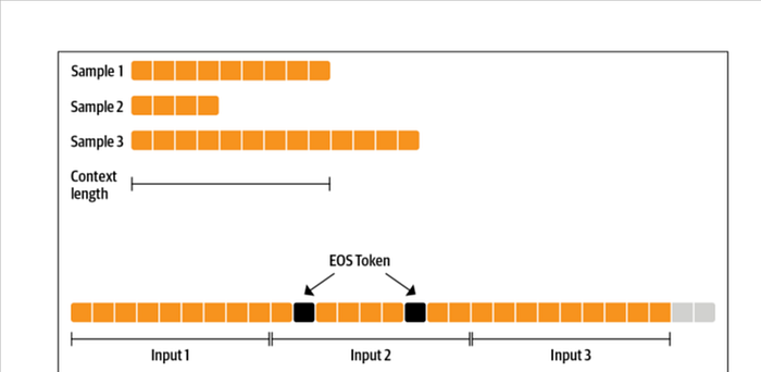
We can, for instance, make sure we have roughly one hundred full sequences in our tokenized examples by defining our input string character length as:

input_characters = number_of_sequences * sequence_length *characters_per_token

where:

• input_characters is the number of characters in the string input to our tokenizer.

• number_of_sequences is the number of (truncated) sequences we would like from our tokenizer, (e.g., 100).

• sequence_length is the number of tokens per sequence returned by the token‐ izer, (e.g., 1,024).

• characters_per_token is the average number of characters per output token that we first need to estimate.

By feeding the tokenizer a string containing input_characters characters, we can expect it to yield approximately number_of_sequences output sequences. This setup also allows us to quantify any potential data loss from truncation. For instance, if number_of_sequences is set to 100, we're essentially segmenting the input into 100 sequences and discarding at most one incomplete sequence at the end. This results in a maximum loss of around 1% of the dataset. Importantly, this method helps maintain the integrity of the dataset by avoiding systematic trimming of file endings, which could otherwise introduce bias.

Let's first estimate the average character length per token in our dataset:

examples, total_characters, total_tokens = 500, 0, 0
dataset = load_dataset('transformersbook/codeparrot-train', split='train',
 streaming=True)
for _, example in tqdm(zip(range(examples), iter(dataset)), total=examples):
 total_characters += len(example['content'])
 total_tokens += len(tokenizer(example['content']).tokens())
characters_per_token = total_characters / total_tokens
print(characters_per_token)

#output
3.6233025034779565

We just need to inherit from IterableDataset and set up the __iter__() function that yields the next element with the logic we just walked through:

import torch
from torch.utils.data import IterableDataset
class ConstantLengthDataset(IterableDataset):
 def __init__(self, tokenizer, dataset, seq_length=1024,
 num_of_sequences=1024, chars_per_token=3.6):
 self.tokenizer = tokenizer
 self.concat_token_id = tokenizer.eos_token_id
 self.dataset = dataset
 self.seq_length = seq_length
 self.input_characters = seq_length * chars_per_token * num_of_sequences
 def __iter__(self):
 iterator = iter(self.dataset)
 more_examples = True
 while more_examples:
 buffer, buffer_len = [], 0
 while True:
 if buffer_len >= self.input_characters:
 m=f"Buffer full: {buffer_len}>={self.input_characters:.0f}"
 print(m)
 break
 try:
 m=f"Fill buffer: {buffer_len}<{self.input_characters:.0f}"
 print(m)
 buffer.append(next(iterator)["content"])
 buffer_len += len(buffer[-1])
 except StopIteration:
 iterator = iter(self.dataset)
 all_token_ids = []
 tokenized_inputs = self.tokenizer(buffer, truncation=False)
 for tokenized_input in tokenized_inputs["input_ids'"]:
 for tokenized_input in tokenized_inputs:
 all_token_ids.extend(tokenized_input + [self.concat_token_id])
 for i in range(0, len(all_token_ids), self.seq_length):
 input_ids = all_token_ids[i : i + self.seq_length]
 if len(input_ids) == self.seq_length

Let's test our iterable dataset:

shuffled_dataset = dataset.shuffle(buffer_size=100)
constant_length_dataset = ConstantLengthDataset(tokenizer, shuffled_dataset,
 num_of_sequences=10)
dataset_iterator = iter(constant_length_dataset)
lengths = [len(b) for _, b in zip(range(5), dataset_iterator)]
print(f"Lengths of the sequences: {lengths}")

Output:

Fill buffer: 0<36864
Fill buffer: 3311<36864
Fill buffer: 9590<36864
Fill buffer: 22177<36864
Fill buffer: 25530<36864
Fill buffer: 31098<36864
Fill buffer: 32232<36864
Fill buffer: 33867<36864
Buffer full: 41172>=36864
Lengths of the sequences: [1024, 1024, 1024, 1024, 1024]

Defining the Training Loop

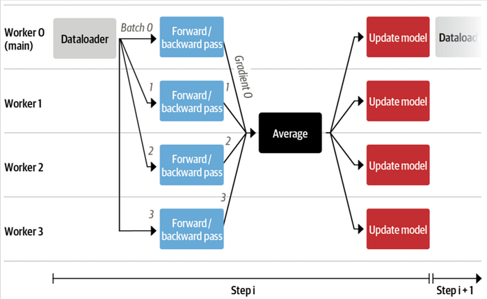
With all components in place, we're ready to implement our training loop. One major challenge when training a language model from scratch — especially at the scale of GPT-2 — is the memory limitation of available GPUs. Even with modern hardware, training such a large model in a reasonable timeframe is not feasible on a single GPU. To address this, we'll adopt data parallelism to leverage multiple GPUs during training. Thankfully, the [Hugging Face] Accelerate library simplifies this process by offering a streamlined API for distributed training. While it's possible to use the Trainer class for this purpose, Accelerate gives us finer control over the training loop—ideal for this hands-on exploration. With Accelerate, the same codebase can effortlessly scale from debugging on a local machine to full-scale training on a powerful multi-GPU or TPU setup. Best of all, adapting a native PyTorch loop for this kind of distributed training only requires a few small adjustments.

 import torch
 import torch.nn.functional as F
 from datasets import load_dataset
+ from accelerate import Accelerator
- device = 'cpu'
+ accelerator = Accelerator()
- model = torch.nn.Transformer().to(device)
+ model = torch.nn.Transformer()
 optimizer = torch.optim.Adam(model.parameters())
 dataset = load_dataset('my_dataset')
 data = torch.utils.data.DataLoader(dataset, shuffle=True)
+ model, optimizer, data = accelerator.prepare(model, optimizer, data)
 model.train()
 for epoch in range(10):
 for source, targets in data:
- source = source.to(device)
- targets = targets.to(device)
 optimizer.zero_grad()
 output = model(source)
 loss = F.cross_entropy(output, targets)
- loss.backward()
+ accelerator.backward(loss)
 optimizer.step()

We set up the hyperparameters for training and wrap them in a Namespace for easy access:

from argparse import Namespace
# Commented parameters correspond to the small model
config = {"train_batch_size": 2, # 12
 "valid_batch_size": 2, # 12
 "weight_decay": 0.1,
 "shuffle_buffer": 1000,
 "learning_rate": 2e-4, # 5e-4
 "lr_scheduler_type": "cosine",
 "num_warmup_steps": 750, # 2000
 "gradient_accumulation_steps": 16, # 1
 "max_train_steps": 50000, # 150000
 "max_eval_steps": -1,
 "seq_length": 1024,
 "seed": 1,
 "save_checkpoint_steps": 50000} # 15000
args = Namespace(**config)

The next step is setting up comprehensive logging for our training process. Since we're training a model from the ground up — a task that is both time-intensive and resource-demanding — it's essential to ensure all key metrics and events are properly tracked. The setup_logging() function establishes three layers of logging: standard Python logging for general output, TensorBoard for visualizing training metrics, and Weights & Biases (W&B) for advanced experiment tracking and collaboration. Depending on your workflow and preferences, you can easily customize this setup to include only the tools you need or integrate additional platforms as necessary.

from torch.utils.tensorboard import SummaryWriter
import logging
import wandb
def setup_logging(project_name):
 logger = logging.getLogger(__name__)
 logging.basicConfig(
 format="%(asctime)s - %(levelname)s - %(name)s - %(message)s",
 datefmt="%m/%d/%Y %H:%M:%S", level=logging.INFO, handlers=[
 logging.FileHandler(f"log/debug_{accelerator.process_index}.log"),
 logging.StreamHandler()])
 if accelerator.is_main_process: # We only want to set up logging once
 wandb.init(project=project_name, config=args)
 run_name = wandb.run.name
 tb_writer = SummaryWriter()
 tb_writer.add_hparams(vars(args), {'0': 0})
 logger.setLevel(logging.INFO)
 datasets.utils.logging.set_verbosity_debug()
 transformers.utils.logging.set_verbosity_info()
 else:
 else:
 tb_writer = None
 run_name = ''
 logger.setLevel(logging.ERROR)

We'll also define a function to log the metrics with TensorBoard and Weights & Biases

 log_metrics(step, metrics):
 logger.info(f"Step {step}: {metrics}")
 if accelerator.is_main_process:
 wandb.log(metrics)
 [tb_writer.add_scalar(k, v, step) for k, v in metrics.items()]

Next, let's write a function that creates the dataloaders for the training and validation sets with our brand new ConstantLengthDataset class:

from torch.utils.data.dataloader import DataLoader
def create_dataloaders(dataset_name):
 train_data = load_dataset(dataset_name+'-train', split="train",
 streaming=True)
 train_data = train_data.shuffle(buffer_size=args.shuffle_buffer,
 seed=args.seed)
 valid_data = load_dataset(dataset_name+'-valid', split="validation",
 streaming=True)
 train_dataset = ConstantLengthDataset(tokenizer, train_data,
 seq_length=args.seq_length)
 valid_dataset = ConstantLengthDataset(tokenizer, valid_data,
 seq_length=args.seq_length)
train_dataloader=DataLoader(train_dataset, batch_size=args.train_batch_size)
 eval_dataloader=DataLoader(valid_dataset, batch_size=args.valid_batch_size)
 return train_dataloader, eval_dataloader

Another aspect we need to implement is optimization

def get_grouped_params(model, no_decay=["bias", "LayerNorm.weight"]):
 params_with_wd, params_without_wd = [], []
 for n, p in model.named_parameters():
 if any(nd in n for nd in no_decay):
 params_without_wd.append(p)
 else:
 params_with_wd.append(p)
 return [{'params': params_with_wd, 'weight_decay': args.weight_decay},
 {'params': params_without_wd, 'weight_decay': 0.0}]

Finally, we want to evaluate the model on the validation set from time to time

def evaluate():
 model.eval()
 losses = []
 for step, batch in enumerate(eval_dataloader):
 with torch.no_grad():
 outputs = model(batch, labels=batch)
 loss = outputs.loss.repeat(args.valid_batch_size)
 losses.append(accelerator.gather(loss))
 if args.max_eval_steps > 0 and step >= args.max_eval_steps: break
 loss = torch.mean(torch.cat(losses))
 try:
perplexity = torch.exp(loss)
 except OverflowError:
perplexity = torch.tensor(float("inf")
return loss.item(), perplexity.item()

Now that we have all these helper functions in place, we are ready to write the heart of the training script:

set_seed(args.seed)
# Accelerator
accelerator = Accelerator()
samples_per_step = accelerator.state.num_processes * args.train_batch_size
# Logging
logger, tb_writer, run_name = setup_logging(project_name.split("/")[1])
logger.info(accelerator.state)
# Load model and tokenizer
if accelerator.is_main_process:
 hf_repo = Repository("./", clone_from=project_name, revision=run_name)
model = AutoModelForCausalLM.from_pretrained("./", gradient_checkpointing=True)
tokenizer = AutoTokenizer.from_pretrained("./")
# Load dataset and dataloader
train_dataloader, eval_dataloader = create_dataloaders(dataset_name)
# Prepare the optimizer and learning rate scheduler
optimizer = AdamW(get_grouped_params(model), lr=args.learning_rate)
lr_scheduler = get_scheduler(name=args.lr_scheduler_type, optimizer=optimizer,
 num_warmup_steps=args.num_warmup_steps,
 num_training_steps=args.max_train_steps,)
def get_lr():
 return optimizer.param_groups[0]['lr']
# Prepare everything with our `accelerator` (order of args is not important)
model, optimizer, train_dataloader, eval_dataloader = accelerator.prepare(
 model, optimizer, train_dataloader, eval_dataloader)
# Train model
model.train()
completed_steps = 0
for step, batch in enumerate(train_dataloader, start=1):
 loss = model(batch, labels=batch).loss
 log_metrics(step, {'lr': get_lr(), 'samples': step*samples_per_step,
 'steps': completed_steps, 'loss/train': loss.item()})
 loss = loss / args.gradient_accumulation_steps
 accelerator.backward(loss)
 if step % args.gradient_accumulation_steps == 0:
 optimizer.step()
 lr_scheduler.step()
 optimizer.zero_grad()
 completed_steps += 1
 if step % args.save_checkpoint_steps == 0:
 logger.info('Evaluating and saving model checkpoint')
 eval_loss, perplexity = evaluate()
 log_metrics(step, {'loss/eval': eval_loss, 'perplexity': perplexity})
 accelerator.wait_for_everyone()
 unwrapped_model = accelerator.unwrap_model(model)
 if accelerator.is_main_process:
 unwrapped_model.save_pretrained("./")
 hf_repo.push_to_hub(commit_message=f'step {step}')
 model.train()
 if completed_steps >= args.max_train_step:
# Evaluate and save the last checkpoint
logger.info('Evaluating and saving model after training')
eval_loss, perplexity = evaluate()
log_metrics(step, {'loss/eval': eval_loss, 'perplexity': perplexity})
accelerator.wait_for_everyone()
unwrapped_model = accelerator.unwrap_model(model)
if accelerator.is_main_process:
 unwrapped_model.save_pretrained("./")
 hf_repo.push_to_hub(commit_message=f'final model')

The Training Run

To streamline the training process, we'll store our training script in a file named codeparrot_training.py, making it easy to run on our training server. Alongside it, we'll include a requirements.txt file that lists all necessary Python dependencies. These files will be added to the model repository on the Hugging Face Hub. Since Hub repositories function like standard Git repositories, we can simply clone the repo, add the required files, and push the changes back. Once everything is in place, initiating the training on our server becomes a simple matter of running a few commands.

$ git clone https://huggingface.co/transformersbook/codeparrot
$ cd codeparrot
$ pip install -r requirements.txt
$ wandb login
$ accelerate config
$ accelerate launch codeparrot_training.py

Our model is now training!

After the full training run completes successfully, you can merge the experiment branch on the Hub back into the main branch with the following commands:

$ git checkout main
$ git merge <RUN_NAME>
$ git push

Results and Analysis

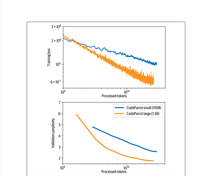
After anxiously monitoring the logs for a week, you will probably see loss and perplexity curves that look like those shown in Figure . The training loss and validation perplexity go down continuously, and the loss curve looks almost linear on the log-log scale. We also see that the large model converges faster in terms of processed tokens, although the overall training takes longer.

In this section, we explore how large language models, specifically fine-tuned on code (like CodeParrot), can be used to assist with software development tasks. We demonstrate how to generate functional code snippets from prompts, evaluate the model both qualitatively and quantitatively, and understand the strengths and limitations of such models through practical examples. We'll begin with hands-on demonstrations and wrap up with insights into evaluating model performance.

Types of Analysis

Qualitative Analysis:

• Involves examining specific, concrete examples.
• Helps understand when the model performs well or poorly.

Quantitative Analysis:

• Uses statistical methods to evaluate performance over a large set of test cases.
• Offers a more robust and systematic view of model capabilities.

Setting Up the Model for Code Generation

• First, we initialize a text-generation pipeline using Hugging Face's transformers library:

from transformers import pipeline, set_seed

model_ckpt = 'transformersbook/codeparrot-small'
generation = pipeline('text-generation', model=model_ckpt, device=0)

• The model generates code until a maximum token length is reached.
• To isolate just the first meaningful output (e.g., a function or class), we define a helper function:

Helper Functions to Format Code Output

import re
from transformers import set_seed

def first_block(string):
    return re.split('\nclass|\ndef|\n#|\n@|\nprint|\nif', string)[0].rstrip()

def complete_code(pipe, prompt, max_length=64, num_completions=4, seed=1):
    set_seed(seed)
    gen_kwargs = {
        "temperature": 0.4,
        "top_p": 0.95,
        "top_k": 0,
        "num_beams": 1,
        "do_sample": True,
    }
    code_gens = pipe(prompt, num_return_sequences=num_completions,
                     max_length=max_length, **gen_kwargs)
    code_strings = []
    for code_gen in code_gens:
        generated_code = first_block(code_gen['generated_text'][len(prompt):])
        code_strings.append(generated_code)
    print(('\n' + '=' * 80 + '\n').join(code_strings))

Let's start with a simple example

Example 1: Calculating Area of a Rectangle

Prompt:

def area_of_rectangle(a: float, b: float):
    """Return the area of the rectangle."""

Model Completions:

return math.sqrt(a * b)
================================================================================
return a * b / 2.0
================================================================================
✅ return a * b
================================================================================
return a * b / a

Example 2: Extracting URLs from HTML

Prompt:

def get_urls_from_html(html):
    """Get all embedded URLs in a HTML string."""

Model Completions:

return [url for url in re.findall(r'<a href="(/[^/]+/[^"]+?)">', html)]
================================================================================
return [url for url in re.findall(r'<a href="(.*?)"', html) if url]
================================================================================
return [url for url in re.findall(r'<a href="(/.*)",', html)]
================================================================================
return re.findall(r'<a href="(.*?)" class="url"[^>]*>', html)

🧪 Tested on Hugging Face's homepage using requests, the function returns both internal and external URLs as expected.

Example 3: Converting Python to NumPy

Prompt:

# a function in native python:
def mean(a):
    return sum(a)/len(a)
# the same function using numpy:
import numpy as np
def mean(a):

Completions:

✅ return np.mean(a)
(repeated across all completions)

📌 The model correctly translates a native Python function to its NumPy equivalent.

Example 4: Building a Scikit-learn Model

Prompt:

X = np.random.randn(100, 100)
y = np.random.randint(0, 1, 100)
# fit random forest classifier with 20 estimators

Completions:

reg = DummyRegressor()
forest = RandomForestClassifier(n_estimators=20)
forest.fit(X, y)
================================================================================
clf = ExtraTreesClassifier(n_estimators=100, max_features='sqrt')
clf.fit(X, y)
================================================================================
clf = RandomForestClassifier(n_estimators=20, n_jobs=n_jobs, random_state=1)
clf.fit(X, y)
================================================================================
✅ clf = RandomForestClassifier(n_estimators=20)
clf.fit(X, y)

🎯 Mostly accurate results, though one completion used a different classifier.

Why BLEU Score Falls Short for Code

• BLEU measures n-gram overlap between generated and reference text.
• In code generation, different variable or function names may still produce correct and functional programs.
• Rigid token overlap metrics like BLEU penalize syntactic variation unnecessarily.
• Thus, BLEU is poorly suited for evaluating code, where semantics matter more than surface forms.

Please Give a Clap if you liked the Story.

Subscribe, to have Stories directly in your Inbox:)

https://medium.com/data-science-collective/optimizing-transformer-models-distillation-quantization-and-onnx-explained-6733b91823cd