(Yes, I tried to generate time-series plots with a AI tool. I'm actually surprised by the result).

Why You Need to be Careful with Time-Series Analysis

Analyzing time-series data is, most of the time, not straightforward.

This kind of data has unique particularities and challenges that aren't typically found with other datasets.

For example, the temporal order of observations must be respected, and when data scientists do not take that into account, it leads to poor model performance or, worse, entirely misleading predictions.

We will address these challenges using a real dataset, ensuring that the results are reproducible through the provided code examples in this article.

Without proper dealing with time-series data, you risk creating a model that appears to work during training but falls apart in real-world applications.

This is because time-series data is fundamentally different — it evolves over time, meaning patterns such as seasonality, trends, and stationarity must not be forgotten!

Neglecting key aspects, such as how to split data while preserving temporal integrity, accounting for seasonality, and how to handle missing values, can result in data leakage or biased model evaluations.

Let's explore these important aspects together.

Hello there!

My name is Sara, and I am a Data Scientist specializing in AI Engineering. I hold a Master's degree in Physics and later transitioned into the exciting world of Data Science.

I write about data science, artificial intelligence, and data science career advice. Make sure to follow me and subscribe to receive updates when the next article is published!

In this article we will cover:

1. Seasonality and Trends: Spotting the Patterns in Your Data
2. Feature Engineering for Time-Series
3. Time-Series Data Splitting — Avoid Data Leakage
4. How to do Cross-Validation with Time-Series Data
5. Stationarity and Transformations
6. Bonus: Detecting and Handling Outliers

Loading the Data

We are going to use Kaggle's Electric Production time-series dataset that can be found and downloaded here.

# Preprocess the data: Convert 'DATE' to datetime and set it as the index
file_path = 'Electric_Production.csv'
df = pd.read_csv(file_path)
df['DATE'] = pd.to_datetime(df['DATE'])
df.set_index('DATE', inplace=True)
df.rename(columns={'IPG2211A2N': 'value'}, inplace=True)

Let's take a look at the data:

# Plot the data
plt.figure(figsize=(10, 6))
plt.plot(df['DATE'], df['value'], label='Electric Production')

# Add titles and labels
plt.title('Electric Production Over Time')
plt.xlabel('Date')
plt.ylabel('Electric Production Value')
plt.xticks(rotation=45)
plt.grid(True)
plt.legend()

# Show the plot
plt.show()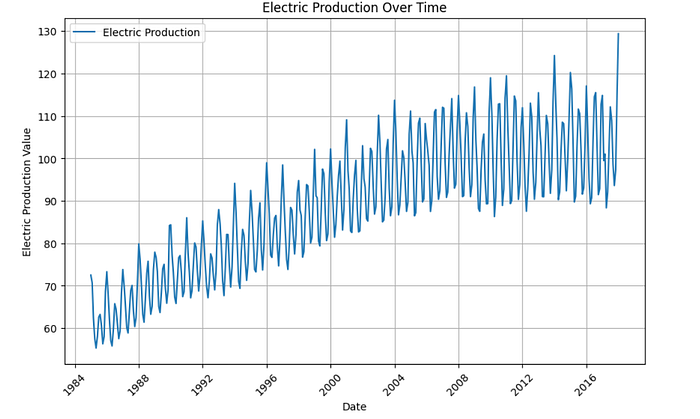

There are many EDA (exploratory data analysis) steps you can take to explore this data, but they are beyond the scope of this article.

Seasonality and Trends: Spotting the Patterns in Your Data

Understanding seasonality and trends is so important in time-series analysis.

What is Seasonality?

Seasonality refers to periodic fluctuations in your data that occur at regular intervals, such as daily, weekly, monthly, or yearly.

For example, retail sales often peak during the holiday season, while electricity consumption may spike during summer months due to air conditioning use.

You need to recognize these seasonal patterns because they can significantly impact your model's predictive power. Ignoring seasonality could lead to poor forecasts and missed opportunities.

Identifying Seasonality

One way to spot seasonality in your data is through visual inspection. Plotting your time-series data can reveal obvious cycles.

However, for a more rigorous approach, you can utilize decomposition techniques. Here's an example using STL decomposition:

from statsmodels.tsa.seasonal import STL
import matplotlib.pyplot as plt

# Assuming 'df' is your DataFrame with a 'value' column
stl = STL(df['value'], seasonal=12)  # Adjust 'seasonal' parameter based on your data
result = stl.fit()
# Extract components
trend = result.trend
seasonal = result.seasonal
residual = result.resid


# Plot the decomposition
plt.figure(figsize=(12, 8))
plt.subplot(411)
plt.plot(df['value'], label='Original Time Series')
plt.legend(loc='upper left')
plt.subplot(412)
plt.plot(trend, label='Trend Component')
plt.legend(loc='upper left')
plt.subplot(413)
plt.plot(seasonal, label='Seasonal Component')
plt.legend(loc='upper right')
plt.subplot(414)
plt.plot(residual, label='Residual Component')
plt.legend(loc='upper right')
plt.tight_layout()
plt.show()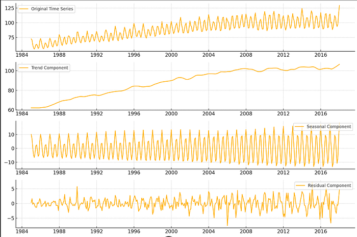

From the image, we can see that the data has a yearly seasonality, with an upward trend. This is common for energy production, which often varies by season.

The seasonal parameter in STL controls the smoothing of the seasonal component. You can adjust this depending on your data's frequency (e.g., monthly, quarterly).

Note: STL assumes that the data points are sequenced in time. STL decomposition expects a series where data points follow one another in their natural temporal order.

Understanding Trends

While seasonality captures predictable fluctuations, trends represent the long-term movement in your data.

A trend can be upward, downward, or flat. Identifying trends is vital because they can influence the overall direction of your forecasts.

For this, you can apply rolling averages to smooth out short-term fluctuations. Here's a quick way to implement that:

# Calculating a 12-month rolling average
df['rolling_avg'] = df['value'].rolling(window=12).mean()

plt.figure(figsize=(10, 5))
plt.plot(df['value'], label='Original Data')
plt.plot(df['rolling_avg'], label='12-Month Rolling Average', color='orange')
plt.title('Original Data vs. Rolling Average')
plt.legend()
plt.show()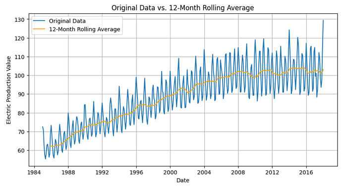

This graph allows you to clearly see the trend amidst seasonal variations, providing a clearer view of the data's overall direction.

A 12-month rolling average will smooth out short-term fluctuations and reveal longer-term trends by averaging the data over a full year (common in time series with seasonality, like this one).

If you want more sensitivity to shorter-term trends without too much smoothing, you can try a 6-month window.

For long-term planning with less noise, a 24-month window may be better.

The Importance of Seasonal and Trend Awareness

Integrating seasonal and trend analysis into your time-series modeling can drastically improve your predictive accuracy.

Additionally, recognizing these patterns helps in feature engineering. You can create features that capture seasonal effects — like month or quarter — as well as lagged variables that account for trends.

This can enhance your model's understanding of the data, and ultimately leading to better predictions!

Understanding Stationarity in Time-Series Data: Key Transformations Explained

Let's explore another crucial aspect of time-series analysis that often trips up even seasoned data scientists: stationarity.

What's the Big Deal with Stationarity?

Stationarity is like the zen state of your time-series data.

It means that the statistical properties of your data — like mean and variance — don't change over time.

Why is this important?

Well, many time-series models assume that your data is stationary. If it's not, your model might not be reliable at all.

Here is an example of how you could check for stationarity:

from statsmodels.tsa.stattools import adfuller

def check_stationarity(timeseries):
    result = adfuller(timeseries, autolag='AIC')
    return result[1]  # Return the p-value
# Assuming 'df' is your DataFrame with multiple columns
for column in df.columns:
    p_value = check_stationarity(df[column])
    print(f"Column '{column}': p-value = {p_value}")
    if p_value <= 0.05:
        print(f"  The series '{column}' is likely stationary")
    else:
        print(f"  The series '{column}' is likely non-stationary")
    print()

It printed:

Column 'value': p-value = 0.18621469116586592
The series 'value' is likely non-stationary

Here we are employing the ADF Test.

Very broadly, the ADF test examines whether a time-series is stationary by testing the null hypothesis that a unit root is present in the series, which would indicate non-stationarity.

In this case, the dataset is non-stationary.

If your dataframe has multiple columns that you want to test, you'd need to apply the test to each column separately.

If the p-value is less than 0.05, great! Your data is likely stationary. If not, don't panic — there are solutions.

Transforming Non-Stationary Data

If your data isn't stationary, here are some common transformations you can try:

1. Differencing: Subtract each observation from the previous one.

df['diff'] = df['value'].diff()

By applying differencing, the resulting diff column removes the trend, making the series closer to stationary, which is ideal for many forecasting models.

2. Log Transformation: Great for data with exponential trends.

df['log'] = np.log(df['value'])

3. Moving Average: Smooth out short-term fluctuations.

df['MA'] = df['value'].rolling(window=12).mean()

Rechecking for Stationarity After Transformations

After applying transformations to your time-series data, it's crucial to verify if you've achieved stationarity!

print("Stationarity check for original data:")
check_stationarity(df['value'])
print("\nStationarity check after differencing:")
# Drop NaN values before checking for stationarity
check_stationarity(df['diff'].dropna())

Reversing Transformations for Predictions

Now, let's tackle the pro tip about reversing transformations.

When you make predictions using a model trained on transformed data, you need to "undo" these transformations to get meaningful results.

Here's how you might do this (in another dataset that is not ours):

import numpy as np

# Let's say we've trained a model on log-differenced data
# and made some predictions
log_diff_predictions = model.predict(X_test)

# Step 1: Reverse the log transformation
diff_predictions = np.exp(log_diff_predictions)
# Step 2: Reverse the differencing

# We need the last actual value to start the process
last_actual_value = df['value'].iloc[-1]
original_scale_predictions = []
for diff in diff_predictions:
    prediction = last_actual_value + diff
    original_scale_predictions.append(prediction)
    last_actual_value = prediction
# Now 'original_scale_predictions' contains our forecasts 

# in the original scale of our data
print("Original scale predictions:")
print(original_scale_predictions)

In this example, we first reverse the log transformation using np.exp(), then reverse the differencing by cumulatively adding the differences to the last known actual value.

Why is this important? Imagine presenting a sales forecast to your CEO:

"Our model predicts next month's sales will be 1.2."

CEO: "1.2 what? Millions? Thousands?"

You: "Oh, that's the natural log of the difference from last month's sales."

CEO: 😕

Instead, by reversing the transformations, you can confidently say:

"Our model predicts next month's sales will be $4.5 million, an increase of $500,000 from last month."

CEO: 😃

Remember, the goal of data science is to provide actionable insights!

Feature Engineering for Time-Series: Crafting the Perfect Data Recipe

Unlike traditional datasets, where features often remain static, time-series data has unique temporal patterns that must be harnessed to extract insightful features.

In this section, we'll explore some of the most effective techniques.

1. Lag Features: Harnessing the Power of the Past

One of the most straightforward and powerful techniques in time-series feature engineering is the creation of lag features.

These capture past values of the target variable to predict future values. After all, yesterday's trend often gives a strong indication of tomorrow's direction.

For instance, you can incorporate the energy production from the previous months or year, as features can significantly enhance your model's understanding of historical patterns.

df['lag_1'] = df['value'].shift(1)  # Create a lag feature for the previous time step
df['lag_7'] = df['value'].shift(7)  # Create a lag feature for 7 months ago 

The idea is simple: by shifting the time-series data, we provide the model with access to past observations, helping it learn temporal dependencies in the data.

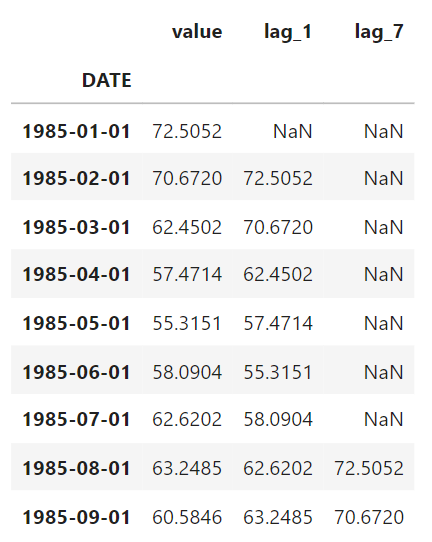
For instance, when you shift the data to create a lag feature (e.g., lag_1), the values from one step before the current row are used as the feature. For the first row of data, however, there is no "previous" row to reference, so the value in the lag_1 column becomes NaN.

2. Rolling Statistics: Smoothing the Noise

Time-series data often exhibits noise, making it harder for models to capture genuine patterns. This is where we employ rolling statistics.

By calculating rolling averages or other metrics (e.g., rolling standard deviation), we can smooth out short-term fluctuations and highlight underlying trends.

For example, to smooth data and observe broader trends, you could calculate a rolling mean over a specified window, such as 12 months:

df['rolling_mean_12'] = df['value'].rolling(window=12).mean()  # 12 months rolling mean
df['rolling_std_24'] = df['value'].rolling(window=12).std()  # 12 months rolling standard deviation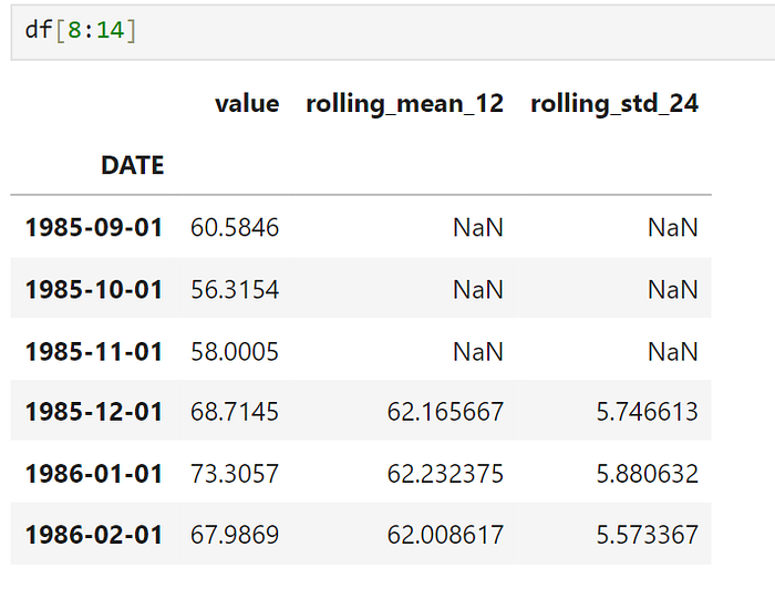

rolling(window=12): This creates a rolling window of 12 time steps (months in this case) to calculate the rolling mean. The same goes for the standard deviation.

With these rolling statistics you get a more stable view of the data, making it easier for your model to pick up on longer-term trends.

3. Date-Time Features: Extracting Temporal Insights

Time-series data concerns not only values changing over time, since it is important to know when those changes occur.

Date-time features such as the hour of the day, day of the week, or month of the year can offer critical insights, especially if your data exhibits seasonal patterns.

You can easily extract such features using Pandas:

df['hour'] = df.index.hour
df['day_of_week'] = df.index.dayofweek
df['month'] = df.index.month
df['year'] = df.index.year   

For the dataset used here, it would make sense to extract the month of the year since monthly data often exhibits seasonal patterns (e.g., higher energy consumption in winter or summer).

These features allow your model to recognize cyclical patterns and seasonal effects, making predictions more reliable.

4. Differences: Tackling Trends and Seasonality

In some cases, your time-series data may exhibit strong trends or seasonality, making it non-stationary.

To handle this, you can create difference features, which capture the changes between consecutive time steps rather than the absolute values. This can help your model focus on changes over time rather than the level of the series itself:

df['diff_1'] = df['value'].diff(1)  # Difference between consecutive observations
df['diff_7'] = df['value'].diff(7)  # Difference between 7 months observations

These difference features can help stabilize the mean of the series, especially when trends or seasonal variations dominate.

5. Cyclic Features: Wrapping Around Periodicity

When dealing with seasonal data, simple numerical representations of time (e.g., month or day) can fail to meet expectations.

For example, the difference between December (month 12) and January (month 1) is just one month in reality, but numerically it appears much larger. To address this, you can create cyclic features by transforming time-related features into sine and cosine functions:

df['sin_month'] = np.sin(2 * np.pi * df['month'] / 12)
df['cos_month'] = np.cos(2 * np.pi * df['month'] / 12)

With this, you allow your model to better understand cyclic relationships in the data, such as seasonal peaks and troughs.

6. External Features: Adding Context to Your Data

Lastly, don't forget that your time-series data doesn't exist in a vacuum!

Often, incorporating external data, such as weather conditions, holidays, or economic indicators, can dramatically improve your model's performance.

For instance, in our data, including temperature data as a feature or the number of daylight hours could give your model a significant edge ( if this data is available).

df['avg_temperature'] = external_weather_data['avg_temp']
df['max_temperature'] = external_weather_data['max_temp']
df['sunlight_hours'] = external_weather_data['sunlight_hours']

These external features provide context that helps your model understand the external factors influencing your time-series data.

Time-Series Data Splitting: How to Avoid Data Leakage in Machine Learning

Data splitting is one of the first steps in any machine learning project, and in time-series analysis, it becomes even more critical.

Unlike traditional datasets where data points are independent, time-series data is sequential, meaning observations are dependent on their previous values.

Randomly splitting this data into training and test sets can lead to data leakage, a where the model gains access to future information during training, resulting in artificially inflated performance metrics.

Sequential Splitting for Time-Series

In time-series data, we need to respect the chronological order of the observations.

The simplest and most effective approach is sequential splitting, where the training set includes data up to a certain time point, and the test set contains all data after that point.

This ensures that the model never has access to future information during training.

How to Split Your Data Sequentially

In this example, we'll create a training set that includes all data points up to a specified date and a test set with the remaining data.

When splitting time-series data, many practitioners use TimeSeriesSplit from the Scikit-learn library:

import matplotlib.pyplot as plt
from sklearn.model_selection import TimeSeriesSplit

# Train Splits Plot with Printed Date Ranges
plt.figure(figsize=(10, 6))

for i, (train_index, test_index) in enumerate(tscv.split(df)):
    train_data, test_data = df.iloc[train_index], df.iloc[test_index]

    # Plot train splits with transparency
    plt.plot(train_data.index, train_data['value'], label=f"Train Split {i+1}", alpha=0.5)

    # Get the train date range
    train_start, train_end = train_data.index[0], train_data.index[-1]

    # Print train date range and number of samples
    print(f"Train Split {i+1}: {train_start.date()} to {train_end.date()} ({len(train_data)} samples)")

plt.title("TimeSeriesSplit - Train Splits")
plt.xlabel("Date")
plt.ylabel("Electric Production Value")
plt.legend()
plt.xticks(rotation=45)
plt.grid(True)
plt.show()

(There is some overlap of data points, that is why the colors do not look the same as in the label).

It prints:

Train Split 1: 1985-01-01 to 1993-04-01 (100 samples)
Train Split 2: 1985-01-01 to 2001-07-01 (199 samples)
Train Split 3: 1985-01-01 to 2009-10-01 (298 samples)
# Test Splits Plot with Printed Date Ranges
plt.figure(figsize=(10, 6))

for i, (train_index, test_index) in enumerate(tscv.split(df)):
    test_data = df.iloc[test_index]

    # Plot test splits with transparency
    plt.plot(test_data.index, test_data['value'], label=f"Test Split {i+1}", linestyle='--', alpha=0.7)

    # Get the test date range
    test_start, test_end = test_data.index[0], test_data.index[-1]

    # Print test date range and number of samples
    print(f"Test Split {i+1}: {test_start.date()} to {test_end.date()} ({len(test_data)} samples)")

plt.title("TimeSeriesSplit - Test Splits")
plt.xlabel("Date")
plt.ylabel("Electric Production Value")
plt.legend()
plt.xticks(rotation=45)
plt.grid(True)
plt.show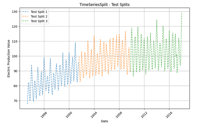

And it prints:

Test Split 1: 1993-05-01 to 2001-07-01 (99 samples)
Test Split 2: 2001-08-01 to 2009-10-01 (99 samples)
Test Split 3: 2009-11-01 to 2018-01-01 (99 samples)

The code uses TimeSeriesSplit from Sklearn to perform time-series splitting, the data into training and test sets while preserving temporal order.

It initializes the splitter with a specified number of splits and iterates through each split to obtain training and test indices. This approach allows for evaluating model performance over different time periods without disrupting the sequence of the data.

How to tweak the n_splits parameter?

• Data Size: Larger datasets can accommodate more splits, while smaller datasets may need fewer splits to ensure each split has enough data.
• Model Evaluation Needs: More splits can provide a more robust evaluation by using different subsets for testing, but may increase computational cost.

On Machine Learning Time-Series: Your Cross-Validation Needs Some Tweaks

Let's talk about why your K-fold cross-validation might be leading you astray when it comes to time series data.

Why Traditional Cross-Validation Does Not Work

Remember how we chatted about the sequential nature of time series data?

Well, this is where it comes back to mess with us in cross-validation.

Your standard K-fold cross-validation assumes that data points are independent and identically distributed (i.i.d.). But in time series, tomorrow depends on today, which depends on yesterday…

Using traditional cross-validation methods can lead to:

1. Data leakage (Your model just saw the future 🔮).
2. Overly optimistic performance estimates.
3. Models that work great in training but flop in the real world.

Time Series Cross-Validation

Time series cross-validation: this technique respects the temporal order of your data.

TimeSeriesSplit creates a fixed number of splits where the training set contains progressively larger data, but each fold tests on a new period without overlapping with the previous test period.

Here's what TimeSeriesSplit does (example):

• Fold 1: Train on [1, 2, 3], Test on [4]
• Fold 2: Train on [1, 2, 3, 4], Test on [5]
• Fold 3: Train on [1, 2, 3, 4, 5], Test on [6]

This makes sure that models are evaluated in a realistic way (training on past data and testing on future data).

In our dataset, there is only one feature column. The value column alone isn't enough because it represents only the current time step at each point, without providing any historical context. Time-series models need to understand how past data influences future outcomes.

Creating features like lagged values (previous observations) or rolling statistics (averages or trends over time) allows the model to learn temporal patterns and relationships.

Let's look at how to implement it:

import pandas as pd
import numpy as np
from sklearn.model_selection import TimeSeriesSplit
import matplotlib.pyplot as plt

# Load the dataset (ensure the 'DATE' column is the index)
df = pd.read_csv('Electric_Production.csv', index_col='DATE', parse_dates=True)

# Create lag features to serve as your feature matrix X
df['lag_1'] = df['value'].shift(1)
df['lag_2'] = df['value'].shift(2)
df['lag_3'] = df['value'].shift(3)

# Drop NaN values due to lagging
df = df.dropna()

# Define X (features) and y (target variable)
X = df[['lag_1', 'lag_2', 'lag_3']]  # Feature matrix: lagged values
y = df['value']  # Target variable

# Apply TimeSeriesSplit
tscv = TimeSeriesSplit(n_splits=5)

# Visualization of Time Series Cross-Validation
fig, ax = plt.subplots(figsize=(10, 5))

for i, (train_index, test_index) in enumerate(tscv.split(X)):
    ax.plot(train_index, [i] * len(train_index), 'b-', label='Train' if i == 0 else '')
    ax.plot(test_index, [i] * len(test_index), 'r-', label='Test' if i == 0 else '')

ax.set_title('Time Series Cross-Validation')
ax.set_xlabel('Sample Index')
ax.set_ylabel('CV Iteration')
ax.legend()
plt.tight_layout()
plt.show()

This code creates a visual representation of how TimeSeriesSplit works. Each fold uses a progressively larger training set and a future time period for testing.

Pro Tips for Time-Series Cross-Validation:

1. Mind the Gap: Consider adding a gap between your training and test sets to simulate real-world forecasting scenarios.

tscv = TimeSeriesSplit(n_splits=5, gap=2)

A gap creates a period between the end of the training data and the start of the test data, so that that the model isn't exposed to data it wouldn't have during actual forecasting.

A gap=2 means that two time steps are skipped between the training and test sets during cross-validation.

2. Seasonal Considerations: If your data has strong seasonality, ensure your training and test sets span full seasonal cycles.

Example

Imagine you are forecasting electricity consumption, which follows a strong annual cycle: demand is higher in the summer due to air conditioning and in the winter due to heating.

If you split your data such that part of the summer is in the training set but the corresponding winter period is in the test set, the model may not learn the full annual seasonality, leading to poor performance.

Example Solution:

• Suppose your data covers 3 years (Jan 2018 — Dec 2020) with monthly readings. If you split the data for training and testing within a single year (e.g., training on Jan-May 2019 and testing on June-Dec 2019), this wouldn't capture the full annual pattern (both summer and winter effects).
• Instead, you would want to train the model on data from full years (e.g., train on 2018 and 2019) and test on a full season or year (e.g., 2020). This way, your model can learn the complete seasonal pattern.

3. Forward-Chaining: For an even more robust approach, try forward-chaining cross-validation:

def forward_chaining(X, n_splits):
    for i in range(n_splits):
        train_end = int(len(X) * (i + 1) / (n_splits + 1))
        yield np.arange(train_end), np.arange(train_end, len(X))

# Usage
for train_index, test_index in forward_chaining(X, n_splits=5):
    X_train, X_test = X[train_index], X[test_index]
    y_train, y_test = y[train_index], y[test_index]
    # Train and evaluate your model hereFigure 7:

Forward-chaining is a time-series cross-validation technique where the training set grows with each split, always including past data, while the test set contains future data.

But, contrary to TimeSeriesSplit, each split trains on progressively larger portions of the dataset, but it uses all the remaining data for testing after the training set, not just a fixed fold.

Time-Series Outliers: When Your Data Decides to Stand Out

Detecting and handling outliers in time-series data is another challenge data scientists face in most projects they work on.

Outliers can bias your analysis, disrupt trends, and negatively affect the accuracy of your model's performance.

Outliers, which are extreme values that deviate from the general pattern of the data, can arise due to various reasons such as sudden economic changes, measurement errors, or rare but important events (like natural disasters).

While it is true that these anomalies can hold valuable insights, they can also mislead models, especially in forecasting tasks.

Identifying Outliers: Distinguishing Signal from Noise

Outliers in time-series data aren't always easy to spot. What appears to be an outlier in a single time step might actually be part of a seasonal pattern or a short-term trend.

Some common methods for detecting outliers in time-series include:

• Moving Averages and Rolling Windows: Sudden deviations from the rolling mean can signal outliers.
• Statistical Tests: Techniques such as the Grubbs' test or Z-scores can be used, but need to account for the sequential nature of the data.
• Visualization: Plotting time-series data is often the best first step to visually inspect for abnormal spikes or dips.

I have written a series of articles regarding outliers in time-series data.

The first article of this series was about exploring both visual and statistical methods to identify outliers effectively in time-series data:

In the second article, we explored several machine learning techniques to identify outliers:

The third article tackled various strategies on how to manage these outliers, considering special factors for time-series data:

I hope these articles come in handy for your outlier hunt!

Final Note

Time-series analysis presents unique challenges that set it apart from traditional machine learning tasks.

In this article, we explored six crucial techniques to optimize your time-series analysis: Time-series data splitting, cross-validation, stationarity, seasonality, feature engineering, and finally, detecting and handling outliers.

Proper data splitting techniques allows you to avoid data leakage, so your model does not have access to the future.

Seasonality is important because it helps identify recurring patterns in the data, which can improve the accuracy of time series forecasting models.

Checking for stationarity and trends is important to make sure your model captures the right patterns and makes accurate predictions.

Cross-validation methods like TimeSeriesSplit and forward-chaining make sure the temporal dependencies are respected.

Feature engineering, including the creation of lag and rolling statistics features, enable us to capture the temporal patterns in the data.

Finally, detecting and addressing outliers makes your model's predictions be reliable.

Ultimately, time-series modeling is about understanding the rhythm of your data, respecting its sequential nature, and making informed decisions that mirror real-world applications.

Stay curious, and happy forecasting! 📈🔮

What other important technique regarding time-series analysis do you use in your daily job? Drop a comment and let me know 😉

If you want to support my work, you can buy me my favorite coffee: a cappuccino. 😊

If you found value in this post, I'd appreciate your support with a clap. You're also welcome to follow me on Medium for similar articles!

Resources:

• LinkedIn

References

TimeSeriesSplit — scikit-learn 1.5.2 documentation

Understanding Stationary Time Series Analysis (analyticsvidhya.com)

11 Classical Time Series Forecasting Methods in Python (Cheat Sheet) — MachineLearningMastery.com

Forecasting: Principles and Practice (3rd ed) (otexts.com)

Time Series Datasets (kaggle.com)