ML Simplified

Machine learning is at the core of modern AI, powering everything from recommendation systems to self-driving cars. But behind every intelligent application lies foundational models that make it all possible. This article provides a concise yet comprehensive breakdown of key machine learning models to help you confidently ace your technical interviews.

Linear Regression

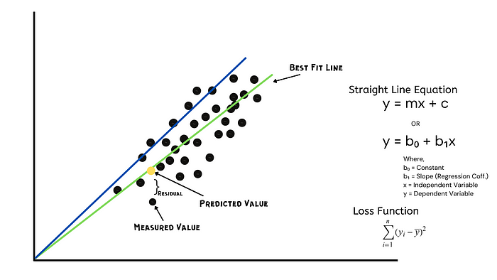
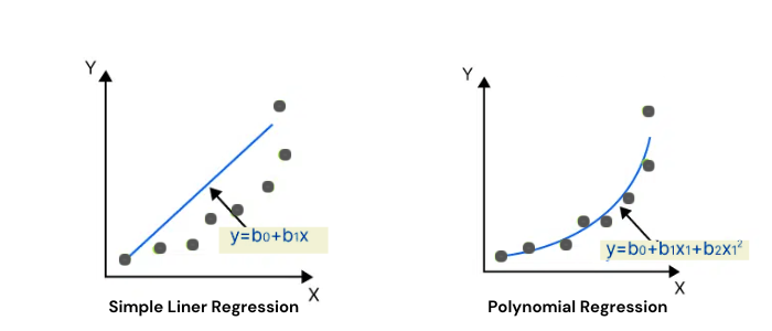
Linear Regression tries to find a relationship between independent and dependent variables by finding a "best-fitted line" that has minimal distance from all the data points using the least square method. The least square method finds a linear equation that minimizes the sum of squared residuals(SSR).

For example, the green line below is a better fit than the blue line because it has a minimal distance from all data points.

Lasso Regression (L1)

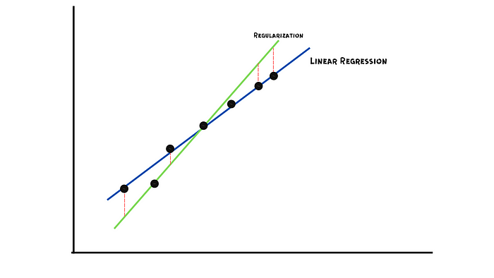
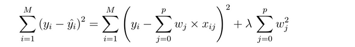
Lasso regression is a regularization technique to reduce overfitting by introducing some amount of bias in the model. It does this by minimizing the squared difference of residual with the addition of a penalty, where the penalty is equal to lambda times the absolute value of the slope. Lambda refers to the severity of the penalty. It works as a hyperparameter that can be changed to reduce overfitting and produce a better fit.

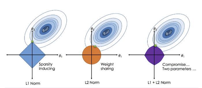
L1 Regularization is a preferred choice when we have a large number of features because it ignores all the variables where the slope value is much less.

Ridge Regression (L2)

Ridge regression is similar to lasso regression. The only difference between the two is the calculation of the penalty term. It adds a penalty term equivalent to the square of the magnitude times lambda.

L2 Regularization is best to use when our data suffers from multicollinearity (independent variables are highly correlated) because it shrinks all the coefficients toward zero.

Elastic Net Regression

Elastic Net Regression combines the penalties from both the lasso and ridge regression to provide a more regularized model.

It allows a balance of both penalties, which results in a better-performing model in comparison to using either l1 or l2 alone.

Polynomial Regression

It models the relationship between the dependent and independent variables as the nᵗʰ degree polynomial. The polynomials are the sum of terms in the form of k.xⁿ, where n is a non-negative integer, k is a constant and x is an independent variable. It is used for non-linear data.

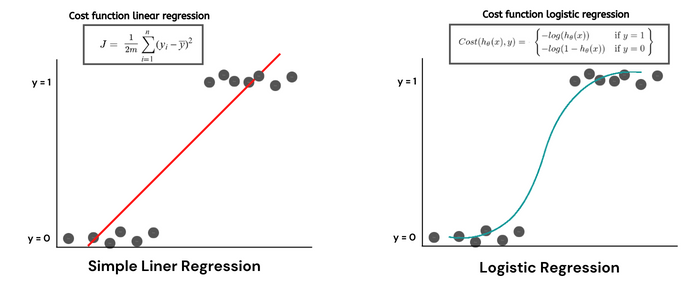
Logistic Regression

Logistic Regression is a classification technique that tries to find the best-fitted curve for data. It makes use of the sigmoid function to convert the output between the range 0 and 1. Unlike linear regression where the best-fitted line is found using the least square method, logistic regression makes use of Maximum Likelihood Estimation (MLE) to find the best-fitted line (curve).

K-Nearest Neighbours (KNN)

KNN is a classification algorithm that classifies new data points based on their distance from the nearest classified points. It assumes that data points exits in close proximity to each other are highly similar.

KNN algorithm is also referred to as a lazy learner because it stores the training data and doesn't classify it into different classes until a new data point occurs for prediction.

By default KNN makes use of Euclidean distance to find the closest classified points for new data, the mode of closest classes is taken to find the predicted class for a new data point.

if the value of k is set to low then a new data point might be considered as an outlier However if it is too high then it may overlook classes with few samples.

Naive Bayes

The Naive Bayes is a classification technique that is based on the Bayes Theorem. It is mostly used for text classification.

Bayes theorem describes the probability of an event, based on prior knowledge of conditions that might be related to the event. It states the following equation —

Naive Bayes is called naive because it assumes that the occurrence of a certain feature is independent of the occurrence of other features.

Support Vector Machines

The goal of support vector machines is to find a hyperplane in an n-dimensional space(n number of features) that can segregate data points into different classes. It is found by maximizing the margin (distance) between the classes.

Support vectors are closed data points to the hyperplane, that can influence the position and orientation of the hyperplane and help maximize the margin between classes. The dimensions of the hyperplane depend upon the number of input features.

Decision Tree

A decision tree is a tree-based structured classifier containing a series of conditional statements that determine what path a sample takes until it reaches the bottom.

The internal nodes of a decision tree represent features, branches represent the decision rule and the leaf node represents the outcome. The decision nodes of the tree work as if-else conditions and leaf nodes contain the output of the decision nodes.

It begins by selecting an attribute as a root node using an attribute selection measure (ID3 or CART), and then recursively comparing the remaining attributes with their parent node to create child nodes until the tree reaches its leaf nodes.

CART (GINI)
1. Probability Table

2. Calculate the Gini Index for Attribute Values Like Overcast, Sunny, Rain
1 - (P/P+N)² -(N/P+N)²

3. Calculate Gini Index for Attribute Eg: Outlook
len(sunny) / len(y) *gini(sunny) + ....

ID3 (INFORMATION GAIN & ENTROPY)
1. Calculate IG For y
IG(Attr) = -[P/P+N] * log[p/P+N] - [N/P+N * log[N/P+N]

2. Calculate Entropy for each value of different attributes in by like outlook - overcase,rain,sunny
entropy(Attr=Value) = -[P/P+N] * log[p/P+N] - [N/P+N * log[N/P+N]

3. Calculte Gain For Attribute Like outlook
Gain(Outlook) = len(sunny) / len(y) *entropy(sunny) + ....

4. Calculate Total Information Gain
IG(y) - Gain(Attribute)
IG(Outcome) - Gain(Outlook)

Random Forest

Random forest is an ensemble technique that consists of several decision trees. It used bagging and feature randomness when building each individual tree to create an uncorrelated forest of decision trees.

Each tree inside a random forest is trained on a different subset of data to predict the outcome, and then the outcome with the majority votes is chosen as random forest prediction.

For example, if we created only one decision tree, the second one, then our prediction will be class 0, but relying on the mode of all four trees our prediction has changed to class 1, This is the power of the random forest.

Extra Trees

Extra Trees is very similar to a random forest classifier the only difference between the two is the way they select root nodes. In a random forest optimal feature is used for splitting, whereas in an Extra tree classifier random feature is selected for the split, the Extra tree provides more randomness and very little correlation between features.

One more comparison between both is that Random Forest uses bootstrap replicas to generate subsets of size N for training ensemble members (Decision trees), whereas Extra Trees use the whole original sample.

The extra tree algorithm is much faster in computation compared to the random forest because the whole procedure of training till prediction is the same for each decision tree considering it randomly chooses the split point.

ADA Boost

ADA Boost is a boosting algorithm that is similar to Random Forest with some significant differences —

1. Rather than building a forest of decision trees, ADA Boost makes a forest of decision stumps. (a stump is a decision tree with only one node and two leaves)
2. Each decision stump is assigned with different weights in final decision-making.
3. It assigns higher weights to data points that are wrongly classified so that they are given more importance while building the next model.
4. It helps combine multiple "Weak Classifiers" into a single strong classifier.

Gradient Boosting

Gradient Boosting builds multiple decision trees where each tree learns from the mistakes of previous trees. It uses residual error to improve the prediction performance. The whole aim of Gradient boosting is to reduce the residual error as much as possible.

Gradient Boosting is similar to ADA Boost, the difference between the two is that ADA Boosts builds decision stumps whereas Gradient Boosting builds decision trees with multiple leaves.

Gradient Boosting starts by building a base decision tree and taking initial predictions usually the average. Then, a new decision tree is created with initial features and residual error as dependent variables. Prediction for the new decision tree is made by taking the initial prediction of the model + the residual error for the sample times learning rate, and the process keeps repeating until we reach minimal error.

K-Means Clustering

KMeans Clustering is an unsupervised machine learning algorithm that groups unlabeled data into K different clusters, where K is a user-defined integer.

It is an iterative algorithm that makes use of cluster centroids to divide the unlabeled data into K clusters in such a way that data points with similar attributes belong to the same cluster.

1. Define K and Create K Clusters
2. Calculate Euclidean Distance of each data point from K Centroid
3. Assing CLosest Data Point to Centroid and Create a CLuster
4. Recalculate Centroid By Taking mean

Hierarchical Clustering

Hierarchical Clustering is another type of clustering-based algorithm that creates a hierarchy of clusters in the form of a tree to divide the data. It automatically finds the relation between data and divides them into n different clusters, where n is the size of the data.

There are two main approaches to hierarchical clustering: agglomerative and divisive.

In agglomerative clustering, we consider each data point as a single cluster and then combine these clusters until we are left with one group (the full dataset). Divisive hierarchical clustering, on the other hand, begins with the whole dataset (considered as one single cluster), which is then partitioned into less similar clusters until each individual data point becomes its own unique cluster.

DBSCAN Clustering

DBSCAN (density-based spatial clustering of application with noise) works upon an assumption that a data point belongs to a cluster if it is closer to many data points of that cluster, rather than any single point.

epsilon and min_points are two important parameters that are useful for dividing data into small clusters. epsilon specifies how close one point should be to another in order to consider it part of the cluster while min_points determining the minimum number of data points required to form a cluster.

Apriori Algorithm

Apriori algorithm is an association rule mining algorithm that maps data items together based on their dependency on each other.

There are some key steps to creating an association rule using the apriori algorithm — 1. Determine support for each item set of size 1, where support is the frequency of items in the dataset. 2. Prone all the items that are below the minimum support threshold (Decided by the user) 3. Create itemset of size n+1 (n is the previous itemset size) and repeat steps 1 and 2, until all itemset support is above a threshold. 4. Generate Rules using confidence (how often x&y occur together when the occurrence of x is already given)

Stratified K-fold Cross-Validation

Stratified K-fold cross-validation is a variation of K-fold cross-validation that uses stratified sampling (rather than random sampling) to create subsets of the data. In stratified sampling, the data is divided into K- number of non-overlapping groups that each have distributions resembling the distribution of the full dataset. Each subset will have an equal number of values for each class label, as demonstrated in the illustration below.

Principle Component Analysis

PCA is a linear dimensionality reduction technique that transforms a set of correlated features into a smaller (k<p) number of uncorrelated features, referred to as principal components. By applying PCA we lose some amount of information but it provides many benefits like improving model performance, reducing hardware requirements, and providing a better opportunity to understand the data using visualization.

Artificial Neural Networks (ANN)

Artificial Neural Networks (ANNs) are inspired by the structure of the human brain, consisting of layers of interconnected neurons. They are composed of an input layer, hidden layers, and an output layer, with each neuron applying weights and activation functions to incoming data. ANNs are widely used for tasks such as image recognition, natural language processing, and predictive analytics due to their ability to learn complex patterns from data.

Convolutional Neural Networks (CNN)

Convolutional Neural Networks (CNNs) are a special type of neural network designed primarily for image and video processing. Unlike traditional neural networks, which treat each pixel as a separate input, CNNs use convolutional layers to scan over images and detect patterns like edges, textures, and shapes. This makes them highly effective at recognizing objects in images, even when they appear in different positions. CNNs power technologies like facial recognition, self-driving cars, and medical image analysis by learning to identify patterns in visual data automatically.

Q-Learning

Q-Learning is a reinforcement learning algorithm that helps machines learn by trial and error. It's commonly used in game AI, robotics, and self-learning trading bots. The idea is simple: an "agent" (like a robot or a game character) interacts with an environment, tries different actions, and gets rewards or penalties based on its choices. Over time, it learns the best actions to take in different situations by storing what it learns in something called a Q-table. This technique is widely used in AI systems that need to make decisions autonomously, like self-driving cars navigating traffic or AI-powered game characters learning how to play chess.

Term Frequency-Inverse Document Frequency

TF-IDF is a text analysis algorithm that helps identify important words in a document. It works by counting how often a word appears (Term Frequency, TF) and balancing it with how rare the word is across all documents (Inverse Document Frequency, IDF). This prevents common words like "the" and "is" from being ranked highly, while highlighting more meaningful words. TF-IDF is widely used in search engines (Google, Bing), keyword extraction, and document ranking, helping systems understand which words are most relevant to a given topic.

Latent Dirichlet Allocation (LDA)

Latent Dirichlet Allocation (LDA) is a topic modeling algorithm used to find hidden themes in large collections of text. It assumes that each document is made up of different topics and that each topic is made up of certain words that frequently appear together. LDA is particularly useful in news categorization, research paper classification, and analyzing customer reviews because it helps uncover the underlying themes in large amounts of unstructured text. If you've ever seen an automatic topic-suggestion feature in a research tool, there's a good chance it's using LDA to group similar texts together.

Word2Vec

Word2Vec is an NLP algorithm that helps computers understand the meaning of words by converting them into numerical vectors. Unlike older methods like TF-IDF, which only look at word frequency, Word2Vec captures semantic relationships between words. For example, it can learn that "king" and "queen" are related, or that "Paris" is to "France" what "Berlin" is to "Germany". This makes it incredibly useful in chatbots, sentiment analysis, and recommendation systems, where understanding word meaning and context is crucial. Many modern language models, including those used in Google Translate and voice assistants, rely on Word2Vec as a foundation for deeper language understanding.

Thanks For Reading Till Here, If You Like My Content and Want To Support Me The Best Way is —

1. Leave a few Claps👋and your thoughts 💬 below.️
2. Follow Me On Medium.
3. Connect With Me On LinkedIn.
4. Attach yourself to My Email List to never miss reading another article of mine