

These last weeks I´ve been reading a lot about the term State Space Model. Mainly because of the famous paper Mamba, this concept is getting very popular in machine learning.
I already knew from my physics classes, that this was a simple approach to solving 'dynamic systems'. But when I started to look at it on the internet I contoured all types of terrific definitions such as:
State-space models are models that use state variables to describe a
system by a set of first-order differential equations,
rather than by one or more nth-order difference equations. [1]
Or others like:
State space modeling is an established framework for analyzing stochastic
and deterministic dynamical systems that are measured or observed through
a stochastic process. [2]
These are definitely not wrong, but perhaps someone who doesn´t have a background in calculus or statistics will think SSMs are very challenging concepts; when they aren´t.
I mean they are, but at its most basic level everyone should be able to understand the concept (as everything in life, I guess).
In this post, I will explain State Space models from a basic point of view, by the end of it you will not be an expert, but at least you will have a robust idea about why they are a fundamental concept in Machine Learning.
So forget the definitions you have just seen and let´s start with the article!
State-Space Models
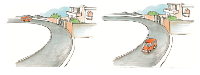
Imagine you have a toy car you can control with a remote, and you want to understand and predict how it moves.
State Space Models (SSMs) are a way to describe this car's movement in terms of two main ideas:
- State
- Observation
The state is like a snapshot of everything you need to know about the car at any moment; where the car is, its direction, how fast it's going…
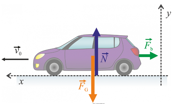
The observation is what you can see or measure about the car. Maybe you can identify its position, but you might not see how fast it's moving.
In simple terms: Think of State Space Models as a way to describe a complex system (like our toy car) in a very organized manner.
By breaking down the system into its state (what's happening inside it) and observations (what can be seen from the outside), we can make predictions about how it will behave in the future.
# But isn´t this the same as any Machine Learning algorithm? We have a set of variables, which we can see and others that we can´t and we have to make a prediction with them about the future state of a system…
Here is where Dynamic systems come into play!
Dynamic vs Static systems
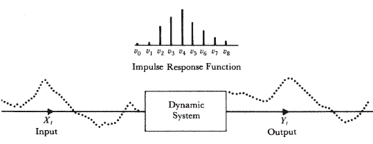
Dynamic systems are characterized by their ability to adapt and evolve over time in response to new data.
They continuously update their models, learning from recent inputs to refine their predictions or behaviors.
In contrast, static systems do not change or adapt once they are deployed. They rely on a fixed model, trained on a pre-defined set of data, and do not incorporate new information or experiences after deployment.
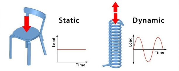
In essence:
Dynamic systems can adjust to changing conditions and new patterns, while static systems are best suited for stable environments with predictable data.
SSMs in machine learning — Time series
In the context of machine learning, state space models are particularly useful in time series analysis which are indeed dynamic systems (change over time).
For example, if we want to create an ML model to classify images into different categories (e.g., dogs, cats, birds) we will use a static system approach as our data won´t change with time
(We might need to modify the algorithm if we get new images but we won´t have to make it adaptable for changes in time).
On the other hand, if our task is to predict the weather, then we will use state-space models which will adapt better to the changes the data will suffer with time.
Mathematical formulation
In mathematical terms, we represent an SSM with a state equation and an observation equation and both of them will be in function of time (t).
But before going through these equations, it´s very important to understand how these models treat time.
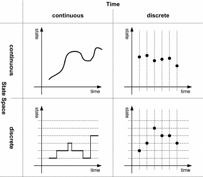
# Time as a discrete variable
State space models analyze time as a discrete variable. This means that it is divided into time steps, which can be hours, days, weeks…
Each time step represents a distinct and separate point in time.
For instance, in a daily model, t = 1 might represent the first day, t = 2 the second day, and so on.
1.- State equation
With this equation, we describe how the state of the system evolves over time (how it varies from one time-step to another).
In its simplest form, it can be written as:
Where:

- `x(t)` is the state vector at time t.

- `A` is the state transition matrix, describing how the state evolves
  from one time step to the next.

- `B` is the input matrix, which maps how inputs u(t) affect the state.

- `w(t)` is the state noise, representing random disturbances or
  modeling errors.
2.- Observation equation
This equation relates the internal state of the system to the observable outputs. It is often represented as:
Where:

- `y(t)` is the output vector at time t.

- `C` is the output matrix, mapping the state to the observed outputs.

- `D` is a matrix that relates the input directly to the output.

- `v(t)` represents the observation noise.
In recap:
The equation contains four main matrices:
# A — The State Transition Matrix This matrix tells us how the current state of the system affects the next state. You can think of it as describing the "rules" that govern the internal mechanics of the system.
For example, if the system is a car, Matrix A would include how the position and velocity of the car will determine its position and velocity a moment later.
# B — The Control Input Matrix This matrix describes how the external inputs or controls you apply affect the state of the system.
It's like the steering wheel, accelerator, and brakes in a car, which dictate how the inputs (like turning the wheel or pressing the pedal) will change the car's speed and direction.
# C — The Output Matrix It tells us what we observe or measure from the system. It translates the state of the system into the outputs or readings that we can see.
Using the car example, Matrix C would include how the car's position and velocity are represented on the car's dashboard gauges.
# D — The Feedforward (or Direct Transmission) Matrix This matrix is a bit less common and is often a matrix of zeros in many systems. It represents any direct relationship between the inputs and the outputs that is not related to the current state.
# And how do we estimate the parameters of the equations?
There are two main ways in which we can determine the parameters of the two equations.
Fundamental principles
We can derive F and H from physical laws or other system-specific principles.
Especially in fields like engineering and physics, the behavior can be described by fundamental principles or laws.
Data fitting
Another option is to make an estimation through empirical data fitting.
I won´t dive too much into this step, but some common methods are:
- Least squares and variants
- Expectation-Maximization (EM) Algorithm
- Maximum Likelihood Estimation (MLE)
# And once you have developed the model how do you make predictions?
Once we have created our state space model we understand how the time steps relate to each other. So by following the model´s "recipe" we can predict the next snapshot by applying the formula we have developed.
However, in real-life conditions, the data is hard to predict and our model may not perform so well.
Estimation algorithms
To improve the accuracy normally we use "tools" that help reduce the bias and keep track of the distribution.
Think of them as smart assistants that help us refine our predictions using our model and new data that comes in.
Probably the most popular one is the Kalman filter.
But there are a lot of them. Some examples are:
- Particle Filters (Sequential Monte Carlo Methods)
- Extended Kalman Filter
- Moving Horizon Estimation (MHE)
- Bayesian Filters
- Least Squares Estimation
Practical example
That has been a lot of theory…
Let´s take a look at our example of forecasting weather with state-space models and put it all together.
We´ll use a set of artificial variables to comprehend the full process.
# Step 1 — Define the observable and state variables
Observable variables
---------------------------------------------------------------------------

- Temperature (Temp)
- Humidity (Hum)
- Barometric pressure (Pres)
- Wind speed and direction (Wind)
These are some examples of variables that we can directly observe and measure.
For instance, temperature can be measured in celsius and humidity in percentages.
State variables
---------------------------------------------------------------------------

- Atmospheric stability (S)
- Moisture content (M)
- Air mass movement (A)
In contrast, state variables cannot be directly measured.
For example, the movement of large bodies of air (air masses), cannot be quantified at a single point.
# Step 2— Define the time steps
In weather forecasting, these could be hourly, daily, or any other relevant interval.
I´ll choose the time steps to update daily, so the collection of all the variables at time t will represent the data collected each day.
# Step 3— Develop the mathematical model
In the first place, I´ll define the observable and state variables vectors (just organizing the variables in a structured way).
Observable variables
State variables
Once we have the variables defined we´ll define the state and observations equations:
State equation
Xt + 1 = F ⋅ Xt + G ⋅ Ut + wt
☣️ Remember:
- F is the state transition matrix that defines how the current state affects
the next state.
- G is the control-input model matrix.Observation equation
Yt = H ⋅ Xt + vt
☣️ Remember:
- H is the observation matrix that maps the state to the observed variables.
- v_t is the observation noise, representing measurement errors and other
uncertainties.Putting all toghether:
Assuming U_t ,w_tand v_tare 0:
# Step 4 — Find F and H
As we discussed before there are two ways in which we can determine this matrices.
- Theoretical modeling (derive F and H from physical laws or other system-specific principle).
- Empirical data fitting (Least Squares, Kalman Filter, Maximum Likelihood Estimation...).
Suppose we construct F based on domain knowledge. It might look something like this:
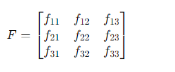
Where:
Each f_{ij} represents the influence of the j-th state variable on the i-th state variable in the next time step. For instance, f_{12} reflects the influence of Atmospheric Stability (S) on Moisture Content (M) from one time step to the next.
The observation matrix might be structured as follows, based on how we believe the latent variables affect the observables:
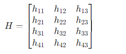
Where
Here, each h_{ij} represents how the j-th state variable affects the i-th observable variable. For example, h_{33} would be how Air Mass Movement (A) affects Barometric Pressure (Pres).
References
[1] https://github.com/rlabbe/Kalman-and-Bayesian-Filters-in-Python