

In the previous parts of the series, I have explained the benefits of keeping track of machine learning experiments and have shown how to do that easily with DVC. One aspect that we have not covered in-depth so far in the series is hyperparameter tuning (HPT).
While some of our experiments might involve changing the dataset, the codebase, adding or removing features, or fixing the odd bug, the number of those will probably still be manageable, as those require us to write code or carry out some analyses manually.
However, this can easily get out of control when we consider hyperparameter tuning. In the previous parts, I showed that with the suggested setup, we can easily control the hyperparameters of the models from the params.yaml file. Additionally, by using DVC, we can easily keep track of the experiments by versioning that file. However, this still involves manually changing the hyperparameters according to our expertise or gut feeling. If we employ a procedure such as grid search, we might fit and evaluate our model thousands of times, each time with a different set of hyperparameters, all in just a few lines of code.
That is why I wanted to show you how we can use the best practices of experiment tracking to also track experiments which are part of an HPT routine.
In case you'd like a refresher on working with DVC, I highly recommend reading the previous parts, as we will not cover all the setup details in this part. You can find the previous articles below:
- Part 1: Turn VS Code into a One-Stop Shop for ML Experiments
- Part 2: Enhance Your ML Experimentation Workflow with Real-Time Plots
- Part 3: The Minimalist's Guide to Experiment Tracking with DVC
- Part 4: Keep Track of Your Backtests with DVC's Experiment Tracking
Setup
For this example, we will work on a sample classification problem using the Default of Credit Card Clients dataset. This dataset contains information on default payments of credit card clients in Taiwan, along with features connected to demographic factors, credit data, history of payment, and bill statements.
As this is a very popular dataset, we will skip exploratory analysis and focus on building and tuning a machine learning model.
Similar to the previous parts, we will be using DVC and its VS Code extension. To keep things simple, we will follow the steps we have taken in the minimalist's approach to experiment tracking. As such, we will focus on tracking our experiments and setting them up. However, I highly encourage you to replicate all the steps we've taken in the previous parts of the series, including setting up data versioning.
The training script
Our starting point will be a training script. In this script, we do a few things:
- We load the data.
- We load the parameters from the
params.yamlfile. - We split the dataset into training and test sets.
- We train a Random Forest classifier using the selected parameters (for simplicity, we only consider the following 3:
class_weight,max_depth,n_estimators). - We store the trained model in the
modelsdirectory. - We track metrics such as accuracy, precision, and recall. Additionally, we also store the confusion matrix and two plots: ROC curve and Precision-Recall curve.
You can find the entire training script below. As you can see, it is quite straightforward. It is essentially the same approach as we have followed in the previous parts of the series.
import json
from pathlib import Path

import pandas as pd
from dvc.api import params_show
from joblib import dump
from sklearn.ensemble import RandomForestClassifier
from sklearn.metrics import accuracy_score, precision_score, recall_score
from sklearn.model_selection import train_test_split

from dvclive import Live
from src.constants import DATA_RAW_DIR, MODELS_DIR, TARGET

# set the params
train_params = params_show()["train"]["params"]

# load data
X = pd.read_csv(f"{DATA_RAW_DIR}/UCI_Credit_Card.csv", index_col="ID")
y = X.pop(TARGET)

# train-test split
X_train, X_test, y_train, y_test = train_test_split(
    X, y, test_size=0.2, random_state=42, stratify=y
)

# fit-predict
model = RandomForestClassifier(random_state=42, **train_params)
model.fit(X_train, y_train)

# store the trained model
model_dir = Path(MODELS_DIR)
model_dir.mkdir(exist_ok=True)

dump(model, f"{MODELS_DIR}/model.joblib")

# get predictions
y_pred = model.predict(X_test)
y_pred_prob = model.predict_proba(X_test)[:, 1]

# tracking the metrics
with Live(save_dvc_exp=True) as live:

    live.log_sklearn_plot("confusion_matrix", y_test, y_pred)
    live.log_sklearn_plot("roc", y_test, y_pred_prob)
    live.log_sklearn_plot("precision_recall", y_test, y_pred_prob)

    metrics = {
        "accuracy": round(accuracy_score(y_test, y_pred), 4),
        "recall": round(recall_score(y_test, y_pred), 4),
        "precision": round(precision_score(y_test, y_pred), 4),
    }

    json.dump(obj=metrics, fp=open("metrics.json", "w"), indent=4, sort_keys=True)
The basics of HPT with DVC
As I have mentioned in the previous parts, it is very easy to manually run an experiment using DVC. Our params.yaml file contains the configuration used by our RF model.
train:
  params:
    class_weight: balanced
    max_depth: 5
    n_estimators: 10
To run an experiment involving changing those values, we could run the following command in our terminal:
dvc exp run --set-param train.params.n_estimators=100Alternatively, we could use the VS Code extension to do the same using prompts in a GUI.
Unfortunately, that approach does not scale well. Now, we will look into alternative methods to make sure that we can explore a wide range of hyperparameters.
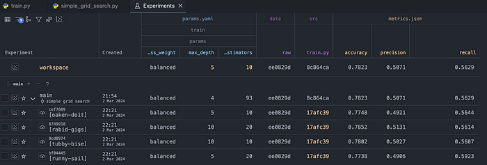
Simple grid search
As our first approach, we will conduct a simple (exhaustive) grid search. That is, we will define a grid of possible hyperparameters and run the training script using all of the possible combinations. To keep it simple, we will test 2 values for n_estimators and max_depth.
In the script below, we execute a command similar to the one mentioned above in a more Pythonic way. First, we instantiate a Repo object. Then, we use it to run experiments. As you can see, we use the same approach to specifying hyperparameters as we have used in the CLI.
To wrap it up, we execute the run method multiple times, each time with a different set of hyperparameters.
import itertools
from dvc.repo import Repo

repo = Repo(".")

# hp grid
n_estimators_grid = [10, 20]
max_depth_grid = [5, 10]

for n_est, max_depth in itertools.product(n_estimators_grid, max_depth_grid):
    repo.experiments.run(
        queue=True,
        params=[
            f"train.params.n_estimators={n_est}",
            f"train.params.max_depth={max_depth}",
        ],
    )
One thing that you probably have noticed is the addition of the queue flag. By including it, we are not immediately running the experiments. We are scheduling them in the queue. That is handy when those experiments might take a long time to run, and we would like to double-check their setup before kicking them off. When we navigate to the Experiments tab in the VS Code extension, we can see the scheduled experiments (with a clock icon next to their names), together with the selected hyperparameters.
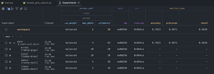
Once we are happy with the setup, we can kick off the queue using the following command:
dvc queue startAfter the experiments are executed, the performance metrics are populated in the table:
Randomized grid search
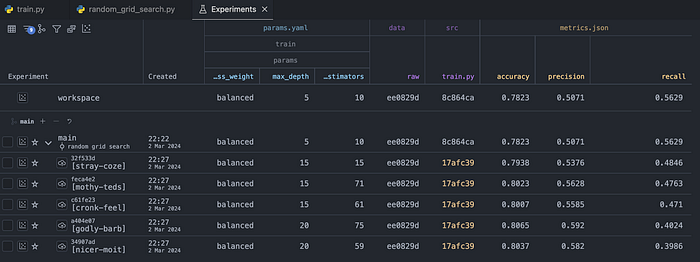
Instead of exhaustively searching through all possible combinations of hyperparameters, we could sample a few random combinations of hyperparameters from the parameter space. This method is especially useful when dealing with a large hyperparameter space, as it can significantly reduce computational cost while still providing good performance.
We execute a randomized search in the following script. As you can see, for the n_estimators, we are sampling random integers from the range 10 to 100. For the max_depth, we are picking one of the 4 predetermined values. We do this for illustration purposes, just to show that we can pick the hyperparameters in multiple ways.
Once again, we are scheduling the experiments in a queue and then manually kicking them off.
import random
from dvc.repo import Repo

repo = Repo(".")

random.seed(0)
N_EXPERIMENTS = 5

for _ in range(N_EXPERIMENTS):

    n_est = random.randint(10, 100)
    max_depth = random.choice([5, 10, 15, 20])

    repo.experiments.run(
        queue=True,
        params=[
            f"train.params.n_estimators={n_est}",
            f"train.params.max_depth={max_depth}",
        ],
    )
Below you can see the results of the randomized search.
Comparing more than the scores
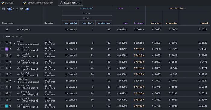
So far, we have used two different approaches to hyperparameter tuning. Using the Experiments tab, we can compare the performance metrics between all of the explored combinations. However, because we also wanted to track some plots in the training script, we can easily delve deeper for a more comprehensive analysis.
To do that, let's pick the best performing model (in terms of recall) from each of the considered grid search approaches. Then, we'll mark them using the little plot icon to the left of their name. By doing so, we indicate which experiments we want to investigate.
After doing that, we navigate to the Plots tab. There, we can inspect the interactive plots that we wanted to track. Using this approach, we can, for example, gain deeper insights into precision and recall by analyzing the curves, instead of just looking at the two sets of numbers.
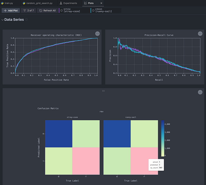
Naturally, we can compare more than two experiments at a time!
Before moving to the next part, it's also worth mentioning that we can easily use the VS Code extension to create custom plots from the metrics stored during our experimentation. To do so, we should scroll to the bottom of the Plots tab where we can find the following pane:

After clicking on the Add Plot button, we will see the following pop-up window that will guide us through the process of creating a custom plot.
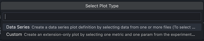
Let's choose the Custom option, and then for the contents of the plot, let's select the max_depth hyperparameter and the tracked recall score.
After selecting these, we can see the following plot, which displays all of the experiments that we have recently run.
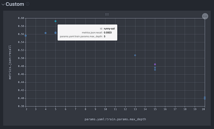
Using custom plots is an alternative and interactive way to explore the contents of the table in the Experiments tab.
Advanced HPT with Optuna
Anytime before you might have thought: "Cool, but there are more advanced HPT methods, for example, the Bayesian Grid Search. Can we do that?" And the answer is: yes, we can! DVC is integrated with Optuna, which is one of the most popular Python libraries for HPT.
To use Optuna's HPT routines, we have to modify our training script. The first difference is that this time we will use 3 sets: training, validation, and test. Training and validation will be used for HPT. After obtaining the best set of hyperparameters, we will once again train the model using training + validation sets and predict using the test set. Strictly speaking, this isn't a must, but it's also a method for testing if overfitting occurred during the hyperparameter tuning stage.
To adapt the code for Optuna, we first create an objective function, which trains the RF model using the selected hyperparameters and returns the recall score on the validation set. Then, we create an Optuna study and indicate that we want to maximize the objective function (in this case, recall).
As I have already mentioned, DVC is integrated with Optuna. To track all the trials of the HPT routine, we just need to add a DVC callback (DVCLiveCallback) to Optuna's optimize method. It's as simple as that!
import json
from pathlib import Path

import optuna
import pandas as pd
import yaml
from dvclive.optuna import DVCLiveCallback
from joblib import dump
from sklearn.ensemble import RandomForestClassifier
from sklearn.metrics import accuracy_score, precision_score, recall_score
from sklearn.model_selection import train_test_split

from dvclive import Live
from src.constants import DATA_RAW_DIR, MODELS_DIR, TARGET


# define the objective function for Optuna
def objective(trial):
    # search space
    n_estimators = trial.suggest_int("n_estimators", 10, 100)
    max_depth = trial.suggest_int("max_depth", 2, 32)
    class_weight = trial.suggest_categorical(
        "class_weight", [None, "balanced", "balanced_subsample"]
    )

    # define and train the RF model with the suggested parameters
    clf = RandomForestClassifier(
        n_estimators=n_estimators, max_depth=max_depth, class_weight=class_weight
    )
    clf.fit(X_train, y_train)

    # Calculate recall on the validation set
    y_pred = clf.predict(X_valid)
    recall = recall_score(y_valid, y_pred)
    return recall


# load data
X = pd.read_csv(f"{DATA_RAW_DIR}/UCI_Credit_Card.csv", index_col="ID")
y = X.pop(TARGET)

# train-valid-test split
X_temp, X_test, y_temp, y_test = train_test_split(
    X, y, test_size=0.2, random_state=42, stratify=y
)

X_train, X_valid, y_train, y_valid = train_test_split(
    X_temp, y_temp, test_size=0.2, random_state=42, stratify=y_temp
)

# Create the Optuna study and optimize the objective function
study = optuna.create_study(direction="maximize")
study.optimize(objective, n_trials=10, callbacks=[DVCLiveCallback()])

# Get the best parameters
best_params = study.best_params
print("Best Parameters:", best_params)

best_params_dict = {"train": {"params": best_params}}

# save the best parameters
with open("params.yaml", "w") as file:
    yaml.dump(best_params_dict, file, default_flow_style=False)


# Train the RandomForestClassifier with the best parameters
best_clf = RandomForestClassifier(**best_params)
best_clf.fit(X_temp, y_temp)

# store the trained model
model_dir = Path(MODELS_DIR)
model_dir.mkdir(exist_ok=True)

dump(best_clf, f"{MODELS_DIR}/model.joblib")

y_pred = best_clf.predict(X_test)
y_pred_prob = best_clf.predict_proba(X_test)[:, 1]

with Live(save_dvc_exp=True) as live:

    live.log_sklearn_plot("confusion_matrix", y_test, y_pred)
    live.log_sklearn_plot("roc", y_test, y_pred_prob)
    live.log_sklearn_plot("precision_recall", y_test, y_pred_prob)

    metrics = {
        "accuracy": round(accuracy_score(y_test, y_pred), 4),
        "recall": round(recall_score(y_test, y_pred), 4),
        "precision": round(precision_score(y_test, y_pred), 4),
    }

    json.dump(obj=metrics, fp=open("metrics.json", "w"), indent=4, sort_keys=True)
After running the modified script, we will see an output in the terminal that will be similar to this one (with different values due to the stochastic component of the search):
[I 2024-03-02 23:05:14,954] A new study created in memory with name: no-name-9d71dba3-4f31-48b4-ac7f-ecd9e556138a
[I 2024-03-02 23:05:16,458] Trial 0 finished with value: 0.4726930320150659 and parameters: {'n_estimators': 56, 'max_depth': 15, 'class_weight': 'balanced'}. Best is trial 0 with value: 0.4726930320150659.
[I 2024-03-02 23:05:18,885] Trial 1 finished with value: 0.3455743879472693 and parameters: {'n_estimators': 42, 'max_depth': 32, 'class_weight': 'balanced'}. Best is trial 0 with value: 0.4726930320150659.
[I 2024-03-02 23:05:22,870] Trial 2 finished with value: 0.3747645951035782 and parameters: {'n_estimators': 93, 'max_depth': 29, 'class_weight': None}. Best is trial 0 with value: 0.4726930320150659.
[I 2024-03-02 23:05:26,376] Trial 3 finished with value: 0.3559322033898305 and parameters: {'n_estimators': 81, 'max_depth': 32, 'class_weight': 'balanced_subsample'}. Best is trial 0 with value: 0.4726930320150659.
[I 2024-03-02 23:05:27,379] Trial 4 finished with value: 0.3267419962335217 and parameters: {'n_estimators': 10, 'max_depth': 28, 'class_weight': 'balanced_subsample'}. Best is trial 0 with value: 0.4726930320150659.
[I 2024-03-02 23:05:30,249] Trial 5 finished with value: 0.3662900188323917 and parameters: {'n_estimators': 64, 'max_depth': 29, 'class_weight': None}. Best is trial 0 with value: 0.4726930320150659.
[I 2024-03-02 23:05:33,264] Trial 6 finished with value: 0.4048964218455744 and parameters: {'n_estimators': 70, 'max_depth': 22, 'class_weight': 'balanced_subsample'}. Best is trial 0 with value: 0.4726930320150659.
[I 2024-03-02 23:05:35,321] Trial 7 finished with value: 0.3615819209039548 and parameters: {'n_estimators': 45, 'max_depth': 30, 'class_weight': 'balanced'}. Best is trial 0 with value: 0.4726930320150659.
[I 2024-03-02 23:05:38,073] Trial 8 finished with value: 0.5028248587570622 and parameters: {'n_estimators': 89, 'max_depth': 13, 'class_weight': 'balanced'}. Best is trial 8 with value: 0.5028248587570622.
[I 2024-03-02 23:05:38,920] Trial 9 finished with value: 0.4745762711864407 and parameters: {'n_estimators': 11, 'max_depth': 16, 'class_weight': 'balanced'}. Best is trial 8 with value: 0.5028248587570622.
Best Parameters: {'n_estimators': 89, 'max_depth': 13, 'class_weight': 'balanced'}
Once we navigate to the Experiments tab, the table will be a bit more complex than before.

That is because we are now tracking two sets of parameters and metrics:
- The contents of the
params.yamlfile and the metrics that are the result of running the script with these values. - The hyperparameters from the Optuna trials, together with the outcome of the objective function.
Okay, let's have a look at the table and unpack what we see there. There's a total of 11 experiments. The first 10 of them (going from the bottom) are the 10 trials of the HPT routine with Optuna. As you can see, the values for the first set of hyperparameters and metrics do not change, only the Optuna variants do.
From the terminal output above, we know that the best trial was the 9th trial (remember about the notation starting with 0!). So the best trial was pawky-dabs.
Then, the pagan-loup experiment is the result of taking the best set of hyperparameters from Optuna and storing them in the params.yaml. Then, we trained the model once again using the training and validation sets and scored on the test set (not seen during HPT). That is also why the recall score from the best trial (pawky-dabs) does not match the recall score from the pagan-loup experiment.
Just as we have done before, we can conduct a deeper analysis by exploring the plots of the particular trials from this group.
Wrapping up
In this article, we explored three automated approaches to hyperparameter tuning. We started by iteratively executing the dvc run exp command to conduct exhaustive and randomized grid search. Afterwards, we used the Optuna library to run Bayesian grid search. Thanks to the DVCLiveCallback, we were able to track all the trials of the HPT routine very easily. Combining this with the knowledge from the previous parts of the series, we can now ensure that all the experiments, including searching for the best set of hyperparameters, are fully reproducible.
On a small side note, I recently gave a presentation at PyData Global about using DVC for experiment tracking. If you are interested, you can check it out here:
You can find the code used in this post in this repository. As always, any constructive feedback is more than welcome. You can reach out to me on LinkedIn, Twitter, or in the comments.
You might also be interested in one of the following:
References
- dataset: https://www.kaggle.com/datasets/uciml/default-of-credit-card-clients-dataset
- Lichman, M. (2013). UCI Machine Learning Repository [http://archive.ics.uci.edu/ml]. Irvine, CA: University of California, School of Information and Computer Science.
All images, unless noted otherwise, are by the author.