

In the world of data-driven decision-making, time series forecasting plays a pivotal role by leveraging historical data patterns to predict future outcomes for several businesses. Whether you are working in asset risk management, trading, weather prediction, energy demand forecasting, or traffic analysis, the ability to forecast accurately is crucial for success.
The success of a time series forecasting project is not measured by only the goodness of fit of forecasting models. The effectiveness of an AI-driven tool in practical application also hinges on the level of collaboration among the diverse actors or instruments involved. To grant the smoothest degree of cooperation, a set of rules and best practices must be introduced as soon as possible starting from the initial developing stages.
These rules are known as Machine Learning Operations (MLOps).
MLOps serves to unify various elements of an ML project into a singular, harmonious structure striving to maintain this seamless integration and functionality in the future.
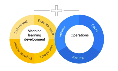
The concept of MLOps is not new in the software development community. It inherits from the DevOps approach the standard phases of a software product release like Continuous Integration (ensure normal running while allowing automatic updates) and Continuous Delivery (automatic deployment); while introducing some specific phases proper of Machine Learning like Continuous Training (automatic feature engineering, parameter tuning, and retraining) and Continuous Monitoring (automatic performances and data drift monitoring).
Nowadays, a lot of tools and frameworks claiming to solve MLOps gaps are present. That's because there is no unique way or architecture for solving MLOps problems. The choices are related to the task to carry out. In the case of time series forecasting, it's important to focus on the temporal dependency present in the data in both the developing and operation phases.
In this post, we provide a practical guide for addressing the requirements of MLOps while executing time series forecasting tasks. We demonstrate how the different elements of machine learning products, dealing with time series, can be replicated using scikit-learn, just like any other tabular machine learning task. This is facilitated through the utilization of tspiral, an open-source Python package designed for time series forecasting with scikit-learn estimators, along with any other library seamlessly compatible with the scikit-learn interface.
DISCLAIMER: I'm the author/developer of tspiral. Many other great open-sourced forecasting packages are available in Python, like Sktime, Darts, or MLForecast (and many more), that can be used to build amazing ML products to solve real-life problems. tspiral was designed to make the smoothest adaptability with the scikit-learn interface. This feature allows the usage of many of the already existing implementations built on top of the scikit-learn ecosystem, reducing the effort for code maintainability, and enhancing the collaboration between people/developers of the open-source community. This post provides examples of how tspiral can be used in various stages of a time forecasting project. The same tasks can also be accomplished using other forecasting tools in different and effective ways.
TRAINING
Whatever predictive model you choose, the training of a scikit-learn model is computed by calling the "fit" attribute and providing a set of predictive features (X) and the corresponding target (y). This smart approach has evolved into a standard within the ML community. Why not apply the same concept to time series forecasting?
from tspiral.forecasting import ForecastingCascade
from sklearn.linear_model import Ridge

forecaster = ForecastingCascade(
    Ridge(),
    lags=range(1,24*7+1),
    groups=[0],
    target_diff=True,
)

forecaster.fit(X=train[['unique_id']], y=train['y'])
In the case of time series forecasting, predictive features are retrieved directly from the target as lagged values. Most forecasting tools automatically generate shifted target values solely based on the input of the target variable rendering, in some cases, the use of additional features (X) unnecessary. On the contrary, passing X, when calling "fit", is mandatory for one-to-one compatibility with scikit-learn.
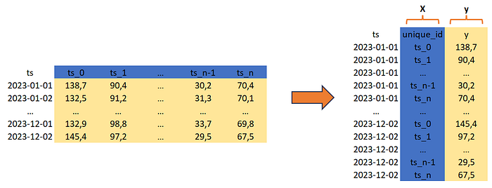
Using columns containing unique integer identifiers enables providing multiple time series forecasting as input while maintaining compatibility with the "fit" method without altering the model's predictive capabilities.
INFERENCE
An ML model trained on a million data points claiming great performance can be nothing if not properly used to make predictions on new data.
When doing inference it's important to reproduce the exact conditions and assumptions made on data during training. Time series data have to maintain a definite temporal order useful to recreate the lagged features based on targets/predictions.
# initialize lag creation from last training samples
preds = forecaster.predict(X=test[['unique_id']])
Most time series forecasting tools use the last training samples to initialize feature lag creation to be used by the trained model when calling "predict". Despite it being a convenient approach, it limits our model to making forecasts only on the same bunch of data, resulting in poor performance in case of future usage or forcing us to carry out additional retraining.
# initialize lag creation from new received data
preds = forecaster.predict(
    X=pd.DataFrame({'unique_id':
                    np.repeat(train['unique_id'].unique(), 24*7)}),
    last_y=train.groupby('unique_id')['y'].head(24*8),
    last_X=train.groupby('unique_id')[['unique_id']].head(24*8)
)
Initializing feature lag creation from newly received data can be a game changer for real-life time series forecasting scenarios, enabling model reuse and optimal monitoring.
EVALUATION
Any ML model must be evaluated on a set of known data before its usage in a production environment. Performances can be computed on a fixed holdout set or through a cross-validation approach. In both cases, it's important to adopt a reliable validation strategy that reflects the usage of our model during inference.

from tspiral.model_selection import TemporalSplit
from sklearn.model_selection import cross_val_score

cv_scores = cross_val_score(
    forecaster,
    X=train[['unique_id']], y=train['y'],
    groups=train[['unique_id']],
    cv=TemporalSplit(n_splits=5, test_size=24*2, gap=24*2),
    scoring='neg_mean_squared_error', error_score='raise',
)
When dealing with multiple time series, it may be useful to consider each time series as a standalone group to maintain temporal fold separation while data may also be unordered.
PARAMETER TUNING
The principles used in performance evaluations can also be applied to parameter tuning. Given an appropriate validation strategy, it's possible to initialize a search of the optimal parameters with any strategy.
from tspiral.model_selection import TemporalSplit
import skopt

model = skopt.BayesSearchCV(
    forecaster,
    search_spaces={
        'estimator__alpha': skopt.space.Real(1,20, prior='log-uniform'),
    },
    cv=TemporalSplit(n_splits=3, test_size=24*2, gap=24*2),
    scoring='neg_mean_squared_error', error_score='raise',
    n_iter=15, random_state=42, refit=True,
).fit(train[['unique_id']], train['y'], groups=train[['unique_id']])
FEATURE SELECTION
Like any other predictive task, also for time series forecasting, it's possible to fulfill feature selection to boost performance or make models lighter. Most feature selection techniques available for standard tabular ML tasks can be applied for time series forecasting.
from tspiral.forecasting import ForecastingCascade
from sklearn.linear_model import Ridge
from sklearn.feature_selection import RFECV
from sklearn.model_selection import ShuffleSplit

forecaster = ForecastingCascade(
    RFECV(
        Ridge(),
        cv=ShuffleSplit(1, test_size=0.25),
        scoring='neg_mean_squared_error',
    ),
    lags=range(1,24*7+1),
    groups=[0],
    target_diff=True,
).fit(train[['unique_id']], train['y'])


feature_ranking = pd.DataFrame({
    'feature': forecaster.feature_names_,
    'ranking': forecaster.estimator_.ranking_,
}).sort_values(by='ranking')
EXPLAINABILITY
In certain situations, the capability to extract insights from a trained model instance can prove immensely advantageous. Nowadays, numerous explainable AI techniques (like SHAP, permutation importance, and many more) are accessible to time series forecasting tasks and can be easily integrated into any machine-learning pipeline.
from tspiral.forecasting import ForecastingCascade
from sklearn.linear_model import Ridge
from sklearn.model_selection import train_test_split
from sklearn.inspection import permutation_importance

class ExplainerRegressor(Ridge):
    def fit(self, X,y):
        id_train, id_val = train_test_split(
            np.arange(X.shape[0]), random_state=42,
        )
        super().fit(X[id_train], y[id_train])

        self.perm_feature_importance_ = permutation_importance(
            self, X[id_val], y[id_val],
            n_repeats=5, random_state=42,
        )['importances_mean']

        return super().fit(X,y)

forecaster = ForecastingCascade(
    ExplainerRegressor(),
    lags=range(1,24*7+1),
    groups=[0],
    target_diff=True,
).fit(train[['unique_id']], train['y'])


feature_importance = pd.DataFrame({
    'feature': forecaster.feature_names_,
    'importance': forecaster.estimator_.perm_feature_importance_,
}).sort_values(by='importance')
PERFORMANCE DRIFT
Performance is nothing without control. Monitoring how the model behaves on new data is fundamental to setting alert thresholds and making decisions accordingly. First of all, if a model is downgrading its performance we can operate a retraining. If the problem persists, we can look at the underlying data for distribution shifts or inspect our pipelines to detect possible bugs.
from tspiral.model_selection import TemporalSplit
from scipy.stats import ks_2samp

CV = TemporalSplit(n_splits=20, test_size=24, gap=24)
stream_simulator = CV.split(train, groups=train['unique_id'])

score_valid, score_test = [], []
for i, (id_past, id_future) in enumerate(stream_simulator):
    if i < 1:
        forecaster.fit(
            X=train[['unique_id']].iloc[id_past],
            y=train['y'].iloc[id_past]
        )
    score = forecaster.score(
        X=train[['unique_id']].iloc[id_future],
        y=train['y'].iloc[id_future],
        last_X=train[['unique_id']].iloc[id_past],
        last_y=train['y'].iloc[id_past],
    )
    if i < CV.get_n_splits() //2:
        score_valid.append(score)
    else:
        score_test.append(score)

ks_2samp(scores_valid, scores_test)
SUMMARY
In this post, we presented a hands-on manual for meeting MLOps prerequisites when performing time series forecasting. We illustrated how to perform different tasks (such as training, inference, evaluation, tuning, …) in a modular way, treating them like in any conventional tabular machine learning application.
Keep in touch: Linkedin