Table of Contents

1. 🌟 Introduction
2. 🔍 Sentinel-2 (Spectral Bands)
3. 🌐 Downloading Sentinel-2 Images
4. ⚙️ Processing Sentinel-2 Images (Clipping and Resampling)
5. 🌋 Visualization of Sentinel-2 Images (Volcano)
6. 🔥 Visualization of Sentinel-2 Images (Wildfire)
7. 📄 Conclusion
8. 📚 References

🌟 Introduction

As you may know, our eyes can only see objects in the visible region (the bands of blue, green, and red). However, when light hits an object and reflects, it contains information in other spectral regions, such as infrared. Infrared light can effectively penetrate and pass through dense gases, such as smoke, providing a clear view beneath the smoke. However, Our eyes are not able to see objects in the infrared region, unlike some animals like snakes that can see a portion of infrared in their vision. During the last decades, there has been significant advancement in the development of sensors for detecting infrared light. These sensors have been used in practical applications.

I have always been looking for a good example to illustrate how satellites can detect crucial information in the infrared region, which is invisible to our naked eyes. Last week, I read about the Iceland volcano that had become active for the third time since December 2023. It sparked an idea in my mind to check the images captured by satellites over the volcano. I hoped to be lucky enough to find a clear satellite image of the smoke plume from the volcano, demonstrating how light scatters in the visible region while penetrating through the smoke in the infrared region to reveal lava flows.

I checked a couple of satellites, and guess what? There was one with the perfect timing! The volcano erupted on Thursday morning (Feb 8th), and the Sentinel-2 overpass occurred on Feb 8th around noon. I thought this could be a perfect example to demonstrate how satellite images, equipped with sensors in the infrared region, can help us monitor a volcano and detect lava even when there is light smoke in the image.

To explore the application of infrared bands in situations with very dense smoke, I decided to visualize another Sentinel-2 image, which captured one of the largest 2020 wildfires in California.

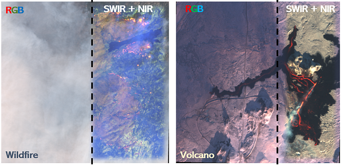
In this story, we will download two Sentinel-2 images, one captured over a volcano on Iceland's Reykjanes Peninsula and the other for the Creek Fire in California in 2020. We will use Python to visualize these two images using different band combinations in the visible and infrared regions. You will see how infrared information can show active lava flows and fire spots, which are obscured in the red, green, and blue (RGB) images. If this sounds interesting to you, read on!

🔍 Sentinel-2 (Spectral Bands)

The Sentinel-2 mission consists of twin satellites, Sentinel-2A and Sentinel-2B developed by the European Space Agency (ESA) as part of the Copernicus Programme. Sentinel-2 satellites have a multispectral instrument that captures data in 13 spectral bands. Each band has a specific wavelength range, allowing for a wide range of Earth observation applications. In this post, we will work with bands in the visible region and three bands in the infrared region. Here is the list of these bands: Band 2 (Blue): 496.6 nm Band 3 (Green): 560.0 nm Band 4 (Red): 664.5 nm Band 8 (NIR — Near Infrared): 835.1 nm Band 11 (SWIR1- Shortwave Infrared): 1613.7 nm Band 12 (SWIR2- Shortwave Infrared): 2202.4 nm

The spatial resolution of Bands 2 (Blue), 3 (Green), 4 (Red), and 8 (NIR) is 10 meters, and Bands 11 and 12 (Shortwave infrared) is 20 meters, which is sufficient to visualize the volcano and wildfires.

🌐 Downloading Sentinel-2 Images

I've already written two tutorials for downloading Sentinel-2 images in Python and R separately. If you want to read the full explanation to know how to sign up, set your credentials, and download images, please refer to the following posts as I discuss the necessary adjustments to the codes for image downloads in this post:

Based on those scripts, you need to modify the coordinates of the area of interest, image dates, and download bands blue, green, red, near-infrared, and shortwave bands for both examples (the volcano and wildfire).

Here are the info that you need for each case:

Iceland Volcano:

satellite = "SENTINEL-2"
level = "S2MSI1C"

aoi_point ="POINT(-22.411503 63.892295)"


start_date = "2024-02-07"
end_date = "2024-02-10"

Creek Fire:

satellite = "SENTINEL-2"
level = "S2MSI1C"

aoi_point ="POINT(-119.26 37.1914)"


start_date = "2020-09-07"
end_date = "2020-09-10"

Once you get a list of available images for the Iceland volcano and the Creek Fire, you will see:

Iceland Volcano:

The volcano eruption happened on Thursday, Feb 8th, 5:30 AM local time and as shown in the screenshot, there is only one image available, captured on February 8th at 13:03 UTC (12:30 local time), exactly 7 hours after the eruption.

Creek Fire:

The Creek Fire began on September 4th and was contained on December 24. Both images in the list were captured on September 8th (4 days after starting wildfire) but the content length of the second image is zero. Therefore, we will work with the first image (S2A_MSIL1C_20200908T183921_N0500_R070_T11SKB_20230309T124945) in this post.

Before running the code for downloading Sentinel-2 images in those two blog posts, make sure that you include three bands in the visible region (Blue, Green, and Red) and three bands in the infrared region (Near-infrared and shortwave infrared bands). The following lines correspond to these bands:

f"{product_name}/{root[0][0][12][0][0][1].text}.jp2" # Blue
f"{product_name}/{root[0][0][12][0][0][2].text}.jp2" # Green
f"{product_name}/{root[0][0][12][0][0][3].text}.jp2" # Red
f"{product_name}/{root[0][0][12][0][0][7].text}.jp2" # Near-infrared
f"{product_name}/{root[0][0][12][0][0][11].text}.jp2" # Shortwave infrared-1
f"{product_name}/{root[0][0][12][0][0][12].text}.jp2" # Shortwave infrared-2

If you have followed the steps correctly, you should have these files for each example in your directory:

Iceland Volcano:

Creek Fire:

⚙️ Processing Sentinel-2 Images (Clipping and Downscaling)

After downloading those images, we need to clip each band for the area of interest (AOI) around the volcano and the wildfire. Since we have the coordinates for each incident, we can create a buffer polygon (3 km for the volcano and 10 km for the wildfire) using this function:

import math

def calculate_new_coordinates(center_lat, center_lon, distance, bearing):
    # Earth radius in kilometers
    earth_radius = 6371.0

    # Convert coordinates to radians
    center_lat_rad = math.radians(center_lat)
    center_lon_rad = math.radians(center_lon)

    # Calculate new latitude
    new_lat_rad = math.asin(math.sin(center_lat_rad) * math.cos(distance / earth_radius) +
                            math.cos(center_lat_rad) * math.sin(distance / earth_radius) * math.cos(bearing))

    # Calculate new longitude
    new_lon_rad = center_lon_rad + math.atan2(math.sin(bearing) * math.sin(distance / earth_radius) * math.cos(center_lat_rad),
                                              math.cos(distance / earth_radius) - math.sin(center_lat_rad) * math.sin(new_lat_rad))

    # Convert back to degrees
    new_lat = math.degrees(new_lat_rad)
    new_lon = math.degrees(new_lon_rad)

    return new_lon, new_lat 

Use the function above for the Iceland Volcano (AOI):

# Center coordinates
center_lat = 63.892295
center_lon = -22.411503

# Buffer distance in kilometers
buffer_distance = 3

# Calculate coordinates for the four corners
north_lon, north_lat = calculate_new_coordinates(center_lat, center_lon, buffer_distance, 0)
south_lon, south_lat = calculate_new_coordinates(center_lat, center_lon, buffer_distance, math.pi)
east_lon, east_lat = calculate_new_coordinates(center_lat, center_lon, buffer_distance, math.pi / 2)
west_lon, west_lat = calculate_new_coordinates(center_lat, center_lon, buffer_distance, -math.pi / 2)

# Print the coordinates in the desired format
print(f"({west_lon:.4f} {north_lat:.4f}, {east_lon:.4f} {north_lat:.4f}, {east_lon:.4f} {south_lat:.4f}, {west_lon:.4f} {south_lat:.4f}, {west_lon:.4f} {north_lat:.4f})")
# Output:
(-22.4728 63.9193, -22.3502 63.9193, -22.3502 63.8653, -22.4728 63.8653, -22.4728 63.9193)

Use the function above for the Creek Fire (AOI):

# Center coordinates
center_lat = 37.19147
center_lon = -119.261175

# Buffer distance in kilometers
buffer_distance = 10

# Calculate coordinates for the four corners
north_lon, north_lat = calculate_new_coordinates(center_lat, center_lon, buffer_distance, 0)
south_lon, south_lat = calculate_new_coordinates(center_lat, center_lon, buffer_distance, math.pi)
east_lon, east_lat = calculate_new_coordinates(center_lat, center_lon, buffer_distance, math.pi / 2)
west_lon, west_lat = calculate_new_coordinates(center_lat, center_lon, buffer_distance, -math.pi / 2)

# Print the coordinates in the desired format
print(f"({west_lon:.4f} {north_lat:.4f}, {east_lon:.4f} {north_lat:.4f}, {east_lon:.4f} {south_lat:.4f}, {west_lon:.4f} {south_lat:.4f}, {west_lon:.4f} {north_lat:.4f})")
# Output:
(-119.3741 37.2814, -119.1483 37.2814, -119.1483 37.1015, -119.3741 37.1015, -119.3741 37.2814)

Then you can use these coordinates for "aoi_polygon_wkt" to clip the jp2 files as I described them in the section of "Stack, Convert to Geotiff, and Clip it to AOI (TOA)" in this post:

# Volcano: Polygon WKT 
aoi_polygon_wkt = "POLYGON ((-22.4728 63.9193, -22.3502 63.9193, -22.3502 63.8653, -22.4728 63.8653, -22.4728 63.9193))"

# Wildfire: Polygon WKT 
aoi_polygon_wkt = "POLYGON ((-119.3741 37.2814, -119.1483 37.2814, -119.1483 37.1015, -119.3741 37.1015, -119.3741 37.2814))"

With these polygons, we can clip the JP2 files to our AOI. However, before stacking these layers for the visualization part, we need to downscale the shortwave infrared bands from 20m to 10m to be compatible with the size of other bands (blue, green, red, and near-infrared). This can be done with the following function:

import rasterio
from scipy.ndimage import zoom

def downscale_raster(input_path, output_path, scale_factor):
    with rasterio.open(input_path) as src:
        # Read the data
        data = src.read(1)

        # Calculate the new dimensions
        new_height = int(src.height / scale_factor)
        new_width = int(src.width / scale_factor)

        # Use scipy's zoom function for resampling
        resampled_data = zoom(data, 1/scale_factor, order=3)

        # Update metadata for the new raster
        transform = src.transform * src.transform.scale(
            (src.width / resampled_data.shape[1]),
            (src.height / resampled_data.shape[0])
        )

        new_profile = src.profile
        new_profile.update({
            'driver': 'JP2OpenJPEG',
            'height': new_height,
            'width': new_width,
            'transform': transform
        })

        # Write the resampled raster to a new file
        with rasterio.open(output_path, 'w', **new_profile) as dst:
            dst.write(resampled_data, 1)

Then, we can apply this function to downscale the shortwave bands from 20m to 10m for each use case.

Use the function above for the Iceland Volcano:

# Usage
input_band_path_B11 = "/content/T27VVL_20240208T130311_B11.jp2"
output_band_path_B11 = "/content/T27VVL_20240208T130311_B11_resampled.jp2"

input_band_path_B12 = "/content/T27VVL_20240208T130311_B12.jp2"
output_band_path_B12 = "/content/T27VVL_20240208T130311_B12_resampled.jp2"

scale_factor = 1/2  # 20m to 10m

downscale_raster(input_band_path_B11, output_band_path_B11, scale_factor)
downscale_raster(input_band_path_B12, output_band_path_B12, scale_factor)

Use the function above for the Creek Fire:

# Usage
input_band_path_B11 = "/content/T11SKB_20200908T183921_B11.jp2"
output_band_path_B11 = "/content/T11SKB_20200908T183921_B11_resampled.jp2"

input_band_path_B12 = "/content/T11SKB_20200908T183921_B12.jp2"
output_band_path_B12 = "/content/T11SKB_20200908T183921_B12_resampled.jp2"

scale_factor = 1/2  # 20m to 10m

downscale_raster(input_band_path_B11, output_band_path_B11, scale_factor)
downscale_raster(input_band_path_B12, output_band_path_B12, scale_factor)

After these steps, you should have two more files in your directory:

Iceland Volcano:

Creek Fire:

With all bands in the same dimension, we can move forward to generate a stack file based on the section "Stack, Convert to Geotiff, and Clip it to AOI (TOA)" in this post.

🌋 Visualization of Sentinel-2 Images (Volcano)

Now that we have two stacked files, one for the volcano event and the other for the wildfire event, we can plot each one of these using different combinations of bands. Specifically, we will create three plots: one based solely on the visible bands (red, green, blue), another based on a combination of visible and near-infrared bands (green, red, and near-infrared), and a third focused exclusively on the infrared region (near-infrared and shortwave bands) to understand what information we might overlook if we omit data from the infrared region. To generate plots similar to the ones shown below, you can refer to the section 📊 Plot the True Color of the TOA and Surface Reflectance Images in this post.

Iceland Volcano:

This is the image recorded in the visible region, and we can see the lava spread around the volcano (the black pixels), the smoke plume of the volcano, and also some very small red areas showing active lava. As mentioned earlier, light can be easily scattered in the visible band, and that's why we see the smoke plume as white pixels in this image. The scattering of light in the visible range can obscure objects, making it challenging to observe the active lava beneath the smoke. Even when adjusting the gain parameters, which control brightness (gain parameter in the script), we can only see the lava flows moving to the west:

With the adjusted gain parameter in the visible spectrum, you can see the lava moving to the west more clearly. However, we still don't know what's happening below the smoke plume. Let's plot this image again, this time with near-infrared information.

You can now see that there were two flows of active lava at that time: one was heading west, somewhat detectable in the visible range, and the other was moving south, which is revealed through near-infrared light. The southward flow was near Grindavik, a town that had been evacuated since the previous eruption in November.

But the question is: Why can we see the lava in the infrared region even when smoke obscures it?

I touched on this in the introduction, but the main reason behind it is that infrared light has a longer wavelength compared to the visible band. This allows it to pass through fine particles, such as dense gas and smoke, without being scattered, unlike visible bands.

Let's move forward and plot the image again, this time using only infrared bands, specifically the shortwave infrared and near-infrared bands:

As you can see, adding the shortwave infrared added another layer of information to the image. In addition to brighter pixels indicating lava, you can see that the black lava in the first and second images is now divided into two regions: red and black. The red region represents the newly burned area as it reflects more in the shortwave bands, likely containing hot lava, while the rest shows inactive lava.

🔥 Visualization of Sentinel-2 Images (Wildfire)

Similar to the previous section, we will plot the Sentinel-2 image for the wildfire using a combination of bands, including visible bands (red, blue, green), visible and near-infrared bands (green, red, and near-infrared), and infrared bands (shortwave and near-infrared). Let's begin with the visible region:

This is the Sentinel-2 image captured over Creek Fire with the visible bands. As discussed earlier, light can easily scatter in the region, and that's why the only thing visible is a very dense smoke plume rising into the atmosphere from the burning areas. However, as shown in the volcano example, light in the infrared region can penetrate smoke and reveal what is hidden in the visible region. To evaluate the situation in dense smoke, let's plot the image using near-infrared and visible bands to reveal what is happening below the smoke:

Not much difference!!

As illustrated here, in contrast to the volcano situation, near-infrared, similar to the visible bands, has been scattered and was not useful for revealing what's happening beneath the smoke. Since Sentinel-2 has two shortwave infrared bands with longer wavelengths compared to near-infrared, we plot this image one more time using those two shortwave infrared bands and near-infrared while removing any visible bands from the visualization:

Isn't it impressive?

Shortwave infrared bands were able to penetrate the dense smoke and reveal the burning areas (shiny and golden pixels) under the thick smoke layer, which were impossible to see with the visible region alone or even with the combination of visible and near-infrared regions. Locating these burning areas could be crucial for fire management and wildfire monitoring.

As the last step, let's put all these together and plot images for both examples side by side with this template:

import rasterio
import numpy as np
import matplotlib.pyplot as plt

# Plot the stacked image
with rasterio.open("stacked_TOA.tif") as src:
    # Define band indices
    blue_band = 1
    green_band = 2
    red_band = 3
    nir_band = 4
    swir1_band = 5
    swir2_band = 6

    # Read bands
    red = src.read(red_band)
    green = src.read(green_band)
    blue = src.read(blue_band)
    nir = src.read(nir_band)
    swir1 = src.read(swir1_band)
    swir2 = src.read(swir2_band)

    # Apply gain
    gain = 2
    red_n = np.clip(red * gain / 10000, 0, 1)
    green_n = np.clip(green * gain / 10000, 0, 1)
    blue_n = np.clip(blue * gain / 10000, 0, 1)
    nir_n = np.clip(nir * gain / 10000, 0, 1)
    swir1_n = np.clip(swir1 * gain / 10000, 0, 1)
    swir2_n = np.clip(swir2 * gain / 10000, 0, 1)

    # Create different composites
    rgb_composite = np.dstack((red_n, green_n, blue_n))
    nir_composite = np.dstack((nir_n, red_n, green_n))
    swir_composite = np.dstack((swir2_n, swir1_n, nir_n))

    # Plot the composites
    plt.figure(figsize=(24, 8))

    plt.subplot(131)
    plt.title('Red, Green and Blue', fontsize=18, fontweight='bold')
    plt.imshow(rgb_composite)
    plt.axis('off')

    plt.subplot(132)
    plt.title('Near-infrared, Red, Green', fontsize=18, fontweight='bold')
    plt.imshow(nir_composite)
    plt.axis('off')

    plt.subplot(133)
    plt.title('Infrared Bands: Shortwave and Near-infrared', fontsize=18, fontweight='bold')
    plt.imshow(swir_composite)
    plt.axis('off')
    
    # Save the plot
    plt.savefig('composite_plot.png')

    plt.show()

The output will be:

As mentioned in the Sentinel-2 section, this satellite has 13 bands, with 9 of them in the infrared region. We only used three bands from the infrared region to reveal the hidden objects beneath the smoke. Feel free to explore the visualization of lavas or burning areas using other infrared bands, such as red-edge (Band 5, 6, 7, and 8A), and observe how it can impact the results.

📄 Conclusion

The comparison between images — one captured in the visible region and others with infrared bands — has revealed the capability and importance of having eyes and sensors in different electromagnetic spectrums. The additional layer of infrared data enables the clear identification and mapping of active lava flows and burning areas that were invisible in the RGB image. The superior penetration of infrared bands, compared to visible light, allows sensors to detect the presence of objects such as active lava and active fires even when smoke obscures them. This capability enhances our capacity to assess the potential risks of these events and make timely decisions for hazard mitigation.

📚 References

Copernicus Sentinel data [2024] for Sentinel data

Copernicus Service information [2024] for Copernicus Service Information.

📱 Connect with me on other platforms for more engaging content! LinkedIn, ResearchGate, Github, and Twitter.

Here are the relevant posts available through these links: