Data scientists are in the business of decision-making. Our work is focused on how to make informed choices under uncertainty.

And yet, when it comes to quantifying that uncertainty, we often lean on the idea of "statistical significance" — a tool that, at best, provides a shallow understanding.

In this article, we'll explore why "statistical significance" is flawed: arbitrary thresholds, a false sense of certainty, and a failure to address real-world trade-offs.

Most important, we'll learn how to move beyond the binary mindset of significant vs. non-significant, and adopt a decision-making framework grounded in economic impact and risk management.

1. Starting from an example

Imagine we just ran an A/B test to evaluate a new feature designed to boost the time users spend on our website — and, as a result, their spending.

The control group consisted of 5,000 users, and the treatment group included another 5,000 users. This gives us two arrays, named treatment and control, each of them containing 5,000 values representing the spending of individual users in their respective groups.

The first and most natural thing to do is to compare the average spending between the two groups.

np.mean(control) # result: 10.00
np.mean(treatment) # result: 10.49

The control group shows an average spend of $10.00, while the treatment group averages $10.49 — a 5% increase! That sounds promising, doesn't it?

But then comes the famous question:

Is this result statistically significant?

At this point, any data scientist would likely turn to the two cornerstones of the "statistically significant" myth:

• p-value, and
• confidence intervals.

Let's see them separately.

2. P-value

The p-value addresses this question:

If there were no real difference between the two groups, how likely is it that we'd observe a result this extreme?

In other words, we assume for a moment that there is no real difference between the treatment and control groups. Then, we test whether the observed result is too extreme to be attributed to random variation — a kind of proof by contradiction.

If we assume that treatment and control are not different, this means that they are just two samples extracted randomly from the same underlying distribution. So the best proxy we can get for that distribution is by just merging them together into a single array (let's call this new array combined).

combined = np.concatenate([treatment, control])

Now, at this point, we can shuffle this new array and split it into a new treatment and a new control group.

This is just like running a new experiment for free. The only difference with our real A/B test is that now we know for sure that there is no difference between treatment and control.

This is called "permutation test". And we can run this new experiment for free and as many times as we want. This is the beauty of it. Let's repeat this procedure for instance 10,000 times:

permutation_results = []

for _ in range(10_000):
  combined = np.random.permutation(combined)
  permutation_treatment = combined[:len(treatment)]
  permutation_control = combined[-len(control):]
  permutation_results.append(
    np.mean(treatment_combined) - np.mean(control_combined))

This is the equivalent of having run 10,000 "virtual" experiments, knowing that treatment and control come from the same distribution.

So, let's plot a histogram to see the outcome of these 10,000 experiments:

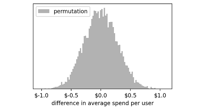
The distribution of these experiments seems centered around zero. This makes a lot of sense because we know that these control and treatment groups are randomly selected from the same array, so most of the time the difference between their averages will be very close to zero.

However, just due to pure chance, there are some extreme cases in which we get large negative or positive numbers: from -$1 to +$1.

In this setting, how likely is it to get a result as extreme as the one we got ($0.49)? To answer this, we just need to compute the percentage of experiments that had an outcome higher than $0.49.

np.mean(np.array(permutation_results) >= 0.49) # result: 0.04

4% of the virtual experiments had an outcome higher than +$0.49.

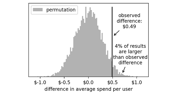
We need to double this number because the result of our real experiment could have been on the left or on the right tail of this histogram. Thus, we get 8%.

This is the number we were looking for: our p-value is 8%.

Is it high? Is it low?

The totally arbitrary rule of thumb that has been used for decades in statistics says that 5% is the threshold we should use. If our p-value is below 5%, then we can conclude that +$0.49 is too extreme to be just random (thus, statistically significant). Otherwise, we can conclude that this number is probably just due to chance (thus, not statistically significant).

Since, in this case, the p-value is 8%, we would conclude that the difference we observed ($0.49) is not statistically significant.

Now let's see how the second tool, the confidence interval, works.

3. Confidence interval

The approach we followed to compute the p-value started by assuming no difference at all between treatment and control. Confidence interval takes the opposite approach.

We assume that the distributions we observed for treatment and control are actually representative of the respective true distributions.

So, just as we did before, we will run a large number of "virtual experiments" by sampling new treatment and control groups from the original data.

The important difference is that we will now draw these samples separately for each group: new treatment samples will be extracted from the original treatment and new control samples will be extracted from the original control.

This means that now we cannot just shuffle the samples, because if we did that the mean of each group wouldn't change!

The really smart trick here is to draw samples with replacement. This mimics the process of drawing new independent samples from the original population and at the same time gives us different samples every time.

This algorithm is called bootstrapping.

Let's run another 10,000 virtual experiments:

bootstrap_results = []

for _ in range(10_000):
  bootstrap_control = np.random.choice(control, size=len(control), replace=True)
  bootstrap_treatment = np.random.choice(treatment, size=len(treatment), replace=True)
  bootstrap_results.append(
    np.mean(bootstrap_treatment) - np.mean(bootstrap_control))

So we now have 10,000 virtual experiments inside the list called bootstrap_results. We can now plot a histogram of these values. And, out of curiosity, let's plot it along with the previous histogram containing the results of the permutation experiments.

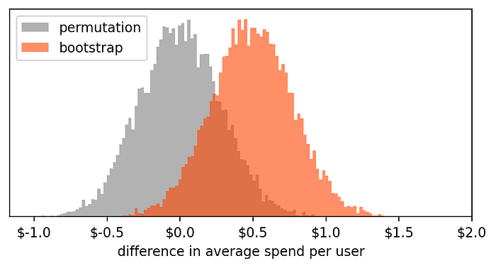
These two histograms tell us two different things:

• Permutation: results of 10,000 virtual tests, assuming that the treatment and control we have observed come from the same population. Thus, any measured difference is just due to chance.
• Bootstrap: results of 10,000 virtual tests, assuming that treatment and control distributions are the ones we observed. Thus, these values approximate the variability in our measure and quantify its uncertainty.

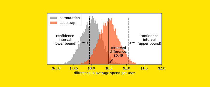
Now, to compute the confidence interval, we'll just have to take two points from the histograms such that 2.5% of the values are on the left and 2.5% of the values are on the right.

This is pretty easy to do with the numpy function percentile.

lower_bound = np.percentile(bootstrap_results, 2.50) # result: -0.0564
upper_bound = np.percentile(bootstrap_results, 97.50) # result: 1.0423

Here is where the interval bounds lie compared to the bootstrap histogram:

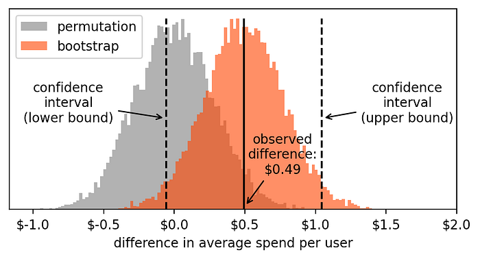
Since the confidence interval includes zero, we must conclude that our result is not statistically significant (i.e. not significantly different from zero).

This makes sense because it is consistent with the information we deduced from the p-value.

4. So what's wrong with "statistical significance"?

In case you had the impression that something is off with the whole procedure of determining statistical significance — I completely agree.

The notion of statistical significance is flawed because of some important reasons:

1. It's awfully arbitrary.
2. It gives a false sense of certainty.
3. It doesn't take risk aversion into account.

Let me explain.

1. It's awfully arbitrary. The threshold typically used to decide on significance is usually 5% or 1%. Why these numbers? For the only reason that they are nice, round numbers. We could easily choose 7% or 0.389% and the theoretical validity would not change.
2. It gives a false sense of certainty. By using a threshold, we give a yes/no answer: significant or not significant. This may give the false impression that the answer is certain. Unfortunately, there's no such thing as certainty in science. All the results lie in a continuum, there's no meaningful threshold.
3. It doesn't take risk aversion into account. The notion of risk aversion is fundamental in decision-making. We know that humans (and companies) prefer to avoid risks as much as possible. P-values and confidence intervals don't account for this at all.

So what? Should we avoid making decisions just because "statistical significance" doesn't work?

Of course not. We should just change the way how we use the tools we have (e.g. the bootstrapping histogram).

5. A better approach to decision-making

Any decision comes with risks and opportunities. And decisions based on data are no exception. So, if we take the example above, what are the risks, and what are the opportunities?

Let's say that we have 1 million users a month. This means that we expect our change to bring around $5.9m in one year (this is $0.49 per user * 1 million users per month * 12 months).

Pretty neat, right? But this is just the expected value and it doesn't tell us the full story. So how could we get the complete picture?

We can compute the economic outcome of each of the 10,000 virtual experiments (that we obtained from bootstrapping) by multiplying its value by 1 million users by 12 months.

For example, if according to a simulated experiment the treatment led to a result of -$0.70 per user, then we know that the overall impact will be-$8.4m (-$0.70 * 1m * 12).

In practice, we can compute the economic impact of each of the 10,000 virtual experiments with this line of code:

# annual impact assuming 1 million users per month
bootstrap_impact = np.array(bootstrap_results) * 1_000_000 * 12

And this is the histogram we get:

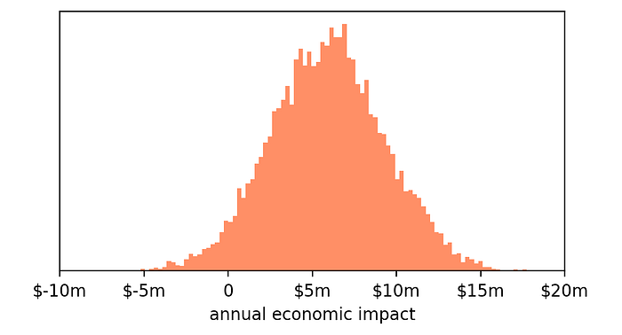
Pretty much what we expected: the average is around +$6m, but we know that due to the variability in our observed results, the outcome can be pretty extreme, for instance -$4m or +$16m.

But we already know that the confidence interval won't tell us much.

So let's go back to the basic notions that are central to decision-making: risks and opportunities. What are the risks and opportunities we are dealing with?

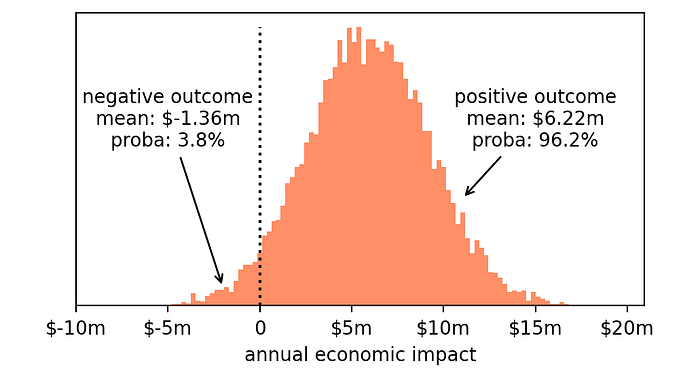
• Risk: losing money. Even if we know that the most likely outcome is +$6m, it may well be that the actual result is an economic loss (indeed, a part of the histogram is to the left of zero).
• Opportunity: gaining money. After all, the majority of the histogram is to the right of zero, so we have a reasonable expectation that this will lead to a positive outcome.

So we can analyze each of these two possibilities and measure how likely they are and what the expected outcome is, in case it comes true.

• Losing money. The probability of losing money if we ship this change is 3.8% and, in this case, we will lose on average $1.36m.
• Gaining money. The probability of a positive outcome is 96.2% and, in this case, we will gain on average $6.22m.

So, is it a good idea to ship this change?

The answer depends on many factors. Considerations like the following. Is this a risk we are willing to run? Or do we prefer to make a new test with more users to reduce the risk? If so, do we have the money and time to run another test? Are there more promising changes we want to test first? And so on.

The point is not what we decide. The point is that we now have better elements to do it. And it's much better to make these trade-offs explicit rather than hiding ourselves behind a simplistic question like: "Is it statistically significant?"

You can reproduce all the code used for this article with this notebook.

Thanks for reading!

If you find my work useful, you can subscribe to receive an email every time that I publish a new article (usually once a month).

Want to show me your support for my work? You can buy me a cappuccino.

If you'd like, follow me on Linkedin!