Outline

1. Introduction
2. When To Use Contextual Bandits 2.1. Contextual Bandit vs Multi-Armed Bandit vs A/B Testing 2.2. Contextual Bandit vs Multiple MABs 2.3. Contextual Bandit vs Multi-Step Reinforcement Learning 2.4. Contextual Bandit vs Uplift Modeling
3. Exploration and Exploitation in Contextual Bandits 3.1. ε-greedy 3.2. Upper Confidence Bound (UCB) 3.3. Thompson Sampling
4. Contextual Bandit Algorithm Steps
5. Offline Policy Evaluation in Contextual Bandits 5.1. OPE Using Causal Inference Methods 5.2. OPE Using Sampling Methods
6. Contextual Bandit in Action
7. Conclusion
8. Acknowledgements
9. References

1. Introduction

Imagine a scenario where you just started an A/B test that will be running for the next two weeks. However, after just a day or two, it is becoming increasingly clear that version A is working better for certain types of users, whereas version B is working better for another set of users. You think to yourself: Perhaps I should re-route the traffic such that users are getting more of the version that is benefiting them more, and less of the other version. Is there a principled way to achieve this?

Contextual bandits are a class of one-step reinforcement learning algorithms specifically designed for such treatment personalization problems where we would like to dynamically adjust traffic based on which treatment is working for whom. Despite being incredibly powerful in what they can achieve, they are one of the lesser known methods in Data Science, and I hope that this post will give you a comprehensive introduction to this amazing topic. Without further ado, let's dive right in!

2. When To Use Contextual Bandits

If you are just getting started with contextual bandits, it can be confusing to understand how contextual bandits are related to other more widely known methods such as A/B testing, and why you might want to use contextual bandits instead of those other methods. Therefore, we start our journey by discussing the similarities and differences between contextual bandits and related methods.

2.1. Contextual Bandit vs Multi-Armed Bandit vs A/B Testing

Let us start with the most basic A/B testing setting that allocates traffic into treatment and control in a static fashion. For example, a data scientist might decide to run an A/B test for two weeks with 50% of traffic going to treatment and 50% going to control. What this means is that regardless of whether we are on the first day of the test or the last, we will be assigning users to control or treatment with 50% probability.

On the other hand, if the data scientist were to use a multi-armed bandit (MAB) instead of an A/B test in this case, then traffic will be allocated to treatment and control in a dynamic fashion. In other words, traffic allocations in a MAB will change as days go by. For example, if the algorithm decides that treatment is doing better than control on the first day, the traffic allocation can change from 50% treatment and 50% control to 60% treatment vs 40% control on the second day, and so on.

Despite allocating traffic dynamically, MAB ignores an important fact, which is that not all users are the same. This means that a treatment that is working for one type of user might not work for another. For example, it might be the case that while treatment is working better for core users, control is actually better for casual users. In this case, even if treatment is better overall, we can actually get more value from our application if we assign more core users to treatment and more casual users to control.

This is exactly where contextual bandits (CB) come in. While MAB simply looks at whether treatment or control is doing better overall, CB focuses on whether treatment or control is doing better for a user with a given set of characteristics. The "context" in contextual bandits precisely refers to these user characteristics and is what differentiates it from MAB. For example, CB might decide to increase treatment allocation to 60% for core users but decrease treatment allocation to 40% for casual users after observing first day's data. In other words, CB will dynamically update traffic allocation taking user characteristics (core vs casual in this example) into account.

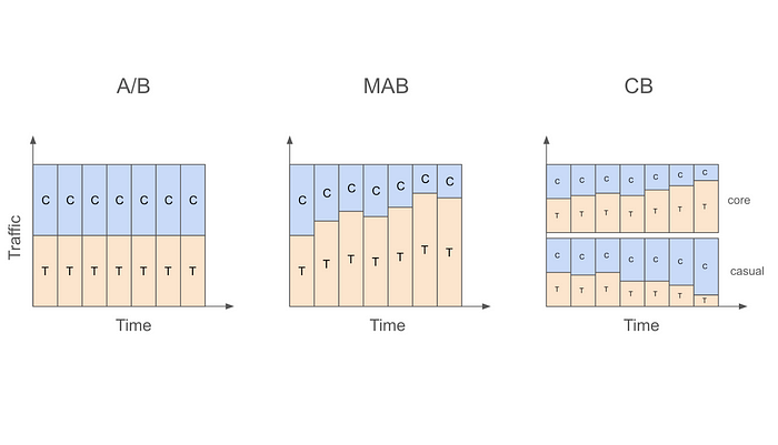
The following table summarizes the key differences between A/B testing, MAB, and CB, and the figure that follows visualizes these ideas.

Table 1: Differences Between A/B Testing, MAB, and CB

Figure 1: Traffic Allocations in A/B Testing, MAB, and CB

2.2. Contextual Bandit vs Multiple MABs

At this point, you might be tempted to think that CB is nothing more than a set of multiple MABs running together. In fact, when the context we are interested in is a small one (e.g., we are only interested in whether a user is a core user or a casual user), we can simply run one MAB for core users and another MAB for casual users. However, as the context gets large (core vs casual, age, country, time since last active, etc.) it becomes impractical to run a separate MAB for each unique context value.

The real value of CB emerges in this case through the use of models to describe the relationship of the experimental conditions in different contexts to our outcome of interest (e.g., conversion). As opposed to enumerating through each context value and treating them independently, the use of models allows us to share information from different contexts and makes it possible to handle large context spaces. This idea of a model will be discussed at several different points in this post, so keep on reading to learn more.

2.3. Contextual Bandit vs Multi-Step Reinforcement Learning

The introduction referred to CB as a class of one-step reinforcement learning (RL) algorithms. So, what exactly is the difference between one-step and multi-step RL? And what makes CB one-step? The fundamental difference between CB and multi-step RL is that in CB we assume the actions the algorithm takes (e.g., serve treatment or control to a specific user) don't affect the future states of the overall system. In other words, the state (or "context" as is more appropriately called in CB) affects what action we take, but that action we took does not in turn impact or change the state. The following figure summarizes this distinction.

Figure 2: Contextual Bandit vs Multi-Step RL

A few examples should make this distinction clearer. Let's say that we are building a system to decide what ads to show to users based on their age. We would expect that users from different age groups may find different ads more relevant to them, which means that a user's age should affect what ads we should show them. However, the ad we showed them doesn't in turn affect their age, so the one-step assumption of CB seems to hold. However, if we move one step further and find out that serving expensive ads deplete our inventory (and limit which ads we can serve in the future) or that the ad we show today affect whether the user will visit our site again, then the one-step assumption is indirectly inviolated, so we may want to consider developing a full-blown RL system instead.

A note of caution though: While multi-step reinforcement learning is more flexible compared to contextual bandits, it's also more complicated to implement. So, if the problem at hand can be accurately framed as a one-step problem (even though it looks like a multi-step problem at first glance), contextual bandits could be the more practical approach.

2.4. Contextual Bandit vs Uplift Modeling

Before moving on to discussing different CB algorithms, I would also like to briefly touch upon the connection between CB and uplift modeling. An uplift model is usually built on top of A/B test data to discover the relationship between the treatment effect (uplift) and user characteristics. The results from such a model can then be used to personalize treatments in the future. For example, if the uplift model discovers that certain users are more likely to benefit from a treatment, then only those types of users might be given the treatment in the future.

Given this description of uplift modeling, it should be clear that both CB and uplift modeling are solutions to the personalization problem. The key difference between them is that CB approaches this problem in a more dynamic way in the sense that personalization happens on-the-fly instead of waiting for results from an A/B test. At a conceptual level, CB can very loosely be thought of as A/B testing and uplift modeling happening concurrently instead of sequentially. Given the focus of this post, I won't be discussing uplift modeling further, but there are several great resources to learn more about it such as [1].

3. Exploration and Exploitation in Contextual Bandits

Above we discussed how CB dynamically allocates traffic depending on whether treatment or control is doing better for a given group of users at a given point in time. This raises an important question: How aggressive do we want to be when we are making these traffic allocation changes? For example, if after just one day of data we decide that treatment is working better for users from the US, should we completely stop serving control to US users?

I'm sure most of you would agree that this would be a bad idea, and you would be correct. The main problem with changing traffic allocations this aggressively is that making inferences based on insufficient amounts of data can lead to erroneous conclusions. For example, it might be that the first day of data we gathered is actually not representative of dormant users and that in reality control is better for them. If we stop serving control to US users after the first day, we will never be able to learn this correct relationship.

A better approach to dynamically updating traffic allocations is striking the right balance between exploitation (serve the best experimental condition based on the data so far) and exploration (continue to serve other experimental conditions as well). Continuing with the previous example, if data from the first day indicate that treatment is better for US users, we can serve treatment to these users with an increased probability the next day while still allocating a reduced but non-zero fraction to control.

There are numerous exploration strategies used in CB (and MAB) as well as several variations of them that try to strike this right balance between exploration and exploitation. Three popular strategies include ε-greedy, upper confidence bound, and Thompson sampling.

3.1. ε-greedy

In this strategy, we first decide which experimental condition is doing better for a given group of users at a given point in time. The simplest way to do this is by comparing the average target values (y) for each experimental condition for these users. More formally, we can decide the "winning" condition for a group of users by finding the condition d that has the higher value for

where n_dx is the number of samples we have so far from users in condition d with context x, and y_idx is the target value for a given sample i in condition d with context x.

After deciding which experimental condition is currently "best" for these users, we serve them that condition with 1-ε probability (where ε is usually a small number such as 0.05) and serve a random experimental condition with probability ε. In reality, we might want to dynamically update our ε such that it is large at the beginning of the experiment (when more exploration is needed) and gradually gets smaller as we collect more and more data.

Additionally, context X might be high-dimensional (country, gender, platform, tenure, etc.) so we might want to use a model to get these y estimates to deal with the curse of dimensionality. Formally, the condition to serve can be decided by finding the condition d that has the higher value for

where x^T is an m-dimensional row-vector of context values and θ_d is an m-dimensional column-vector of learnable parameters associated with condition d.

3.2. Upper Confidence Bound (UCB)

This strategy decides the next condition to serve by looking at not only which condition has a higher y estimate but also our precision of (or confidence in) that estimate. In a simple MAB setting, precision can be thought to be a function of how many times a given condition has already been served so far. In particular, a condition that (i) has a high average y (so it makes sense to exploit) or (ii) has not yet been served many times (so it needs more exploration) is more likely to be served next.

We can generalize this idea to the CB setting by keeping track of how many times different conditions are served in different contexts. Assuming a simple setting with a low-dimensional context X such that CB can be thought of as just multiple MABs running together, we can select the next condition to serve based on which condition d has the higher value for

where c is some constant (to be selected based on how much emphasis we want to put on the precision of our estimate when exploring) and n_x is the number of times context x is seen so far.

However, in most cases, the context X will be high-dimensional, which means that just like in the ε-greedy case, we would need to make use of a model. In this setting, a condition d can be served next if it has the higher value for

where SE(.) is the standard error of our estimate (or more generally a metric that quantifies our current level of confidence in that estimate).

Note that there are several versions of UCB, so you will likely come across different formulas. A popular UCB method is LinUCB that formalizes the problem in a linear model framework (e.g., [2]).

3.3. Thompson Sampling

The third and final exploration strategy to be discussed is Thompson sampling, which is a Bayesian approach to solving the exploration-exploitation dilemma. Here, we have a model f(D, X; Θ) that returns predicted y values given experimental condition D, context X, and some set of learnable parameters Θ. This function gives us access to posterior distributions of expected y values for any condition-context pair, thus allowing us to choose the next condition to serve according to the probability that it yields the highest expected y given context. Thompson sampling naturally balances exploration and exploitation as we are sampling from the posterior and updating our model based on the observations. To make these ideas more concrete, here are the steps involved in Thompson sampling:

In practice, instead of having a single function we can also use a different function for each experimental condition (e.g., evaluate both f_c(X; Θ_c) and f_t(X; Θ_t) and then select the condition with the higher value). Furthermore, the update step usually takes place not after each sample but rather after seeing a batch of samples. For more details on Thompson sampling, you can refer to [3] [4].

4. Contextual Bandit Algorithm Steps

The previous section (especially the part on Thompson sampling) should already give you a pretty good sense of the steps involved in a CB algorithm. However, for the sake of completeness, here is a step-by-step description of a standard CB algorithm:

1. A new data point arrives with context X (e.g., a core user with an iOS device in the US).
2. Given this data point and the exploration strategy chosen (e.g., ε-greedy), the algorithm decides on a condition to serve this user (e.g., treatment or control).
3. After the condition is served, we observe the outcome y (e.g., whether the user made a purchase or not).
4. Update (or fully retrain) the model used in Step 2 after seeing the new data. (As mentioned previously, we usually make an update not after every sample but after seeing a batch of samples to ensure that updates are less noisy.)
5. Repeat.

5. Offline Policy Evaluation in Contextual Bandits

So far we have only discussed how to implement a CB algorithm as new data come in. An equally important topic to cover is how to evaluate a CB algorithm using old (or logged) data. This is called offline evaluation or offline policy evaluation (OPE).

5.1. OPE Using Causal Inference Methods

One way to do OPE is using well-known causal inference techniques such as Inverse Propensity Scoring (IPS) or the Doubly Robust (DR) method. Causal inference is appropriate here because we are essentially trying to estimate the counterfactual of what would have happened if a different policy served a different condition to a user. There is already a great Medium article on this topic [5], so here I will only briefly summarize the main idea from that piece and adapt it to our discussion.

Taking IPS as an example, doing OPE usually requires us to know not only (i) the probability of assigning a given condition to a sample using our new CB algorithm but also (ii) the probability with which a given condition was assigned to a sample in the logged data. Take the following hypothetical logged data with X_1-X_3 being context, D being the experimental condition, P_O(D) being the probability of assigning D to that user, and y being the outcome.

Table 2: Example Logged Data From An A/B Test

As you can see, in this example P_O(D) is always 0.6 for D=1 and 0.4 for D=0 regardless of the context, so the logged data can be assumed to come from an A/B test that assigns treatment with probability 0.6. Now, if we want to test how a CB algorithm would have performed had we assigned conditions using a CB algorithm rather than a simple A/B test, we can use the following formula to get the IPS estimate of the cumulative y for CB

where n is the number of samples in the logged data (which is 5 here) and P_N(D_i) is the probability of serving the logged D for user_i had we used the new CB algorithm instead (this probability will depend on the specific algorithm being evaluated).

Once we have this estimate, we can compare that to the observed cumulative y from the old A/B test (which is 1+0+0+1+1=3 here) to decide if the CB would have yielded a higher cumulative y.

For more information on OPE using causal inference methods, please refer to the article linked at the beginning of the section. The article also links to a nice GitHub repo with lots of OPE implementations.

A side note here is that this section discussed causal inference methods only as a technique used in OPE. However, in reality, one can also apply them while the CB algorithm is being run so as to "debias" the training data that the algorithm collects along the way. The reason why we might want to apply methods such as IPS to our training data is that the CB policy that generates this data is a non-uniform random policy by definition, so estimating causal effects from it to decide what action to take would benefit from using causal inference methods. If you would like to learn more about debiasing, please refer to [6].

5.2. OPE Using Sampling Methods

Another way to do OPE is through the use of sampling methods. In particular, a very simple replay method [7] can be used to evaluate a CB algorithm (or any other algorithm for that matter) using logged data from a randomized policy such as an A/B test. In its simplest form (where we assume a uniform random logging policy), the method works as follows:

1. Sample the next user with context X from the logged data.
2. Decide what condition to assign to that user using the new CB algorithm.
3. If the selected condition matches the actual condition in the logged data, then add the observed y to the cumulative y counter. If it doesn't match, ignore the sample.
4. Repeat until all samples are considered.

If the logging policy doesn't assign treatments uniformly at random, then the method needs to be slightly modified. One modification that the authors themselves mention is to use rejection sampling (e.g., [8]) whereby we would accept samples from the majority treatment less often compared to the minority treatment in Step 3. Alternatively, we could consider dividing the observed y by the propensity in Step 3 to similarly "down-weight" the more frequent treatment and "up-weight" the less frequent one.

In the next section, I employ an even simpler method in my evaluation that uses up- and down-sampling with bootstrap to transform the original non-uniform data into a uniform one and then apply the method as it is.

6. Contextual Bandit in Action

To demonstrate contextual bandits in action, I put together a notebook that generates a simulated dataset and compares the cumulative y (or "reward") estimates for new A/B, MAB, and CB policies evaluated on this dataset. Many parts of the code in this notebook are taken from the Contextual Bandits chapter of an amazing book on Reinforcement Learning [9] (highly recommended if you would like to dig deeper into Reinforcement Learning using Python) and two great posts by James LeDoux [10] [11] and adapted to the setting we are discussing here.

The setup is very simple: The original data we have comes from an A/B test that assigned treatment to users with probability 0.75 (so not uniformly at random). Using this randomized logged data, we would like to evaluate and compare the following three policies based on their cumulative y:

1. A new A/B policy that randomly assigns treatment to users with probability 0.4.
2. A MAB policy that decides what treatment to assign next using an ε-greedy policy that doesn't take context X into account.
3. A CB policy that decides what treatment to assign next using an ε-greedy policy that takes context X into account.

I modified the original method described in the Li et al. paper such that instead of directly sampling from the simulated data (which is 75% treatment and only 25% control in my example), I first down-sample treatment cases and up-sample control cases (both with replacement) to get a new dataset that is exactly 50% treatment and 50% control.

The reason why I start with a dataset that is not 50% treatment and 50% control is to show that even if the original data doesn't come from a policy that assigns treatment and control uniformly at random, we can still work with that data to do offline evaluation after doing up- and/or down-sampling to massage it into a 50/50% dataset. As mentioned in the previous section, the logic behind up- and down-sampling is similar to rejection sampling and the related idea of dividing the observed y by the propensity.

The following figure compares the three policies described above (A/B vs MAB vs CB) in terms of their cumulative y values.

Figure 3: Cumulative Reward Comparison

As can be seen in this figure, cumulative y increases fastest for CB and slowest for A/B with MAB somewhere in between. While this result is based on a simulated dataset, the patterns observed here can still be generalized. The reason why A/B testing isn't able to get a high cumulative y is because it isn't changing the 60/40% allocation at all even after seeing sufficient evidence that treatment is better than control overall. On the other hand, while MAB is able to dynamically update this traffic allocation, it is still performing worse than CB because it isn't personalizing the treatment vs control assignment based on the context X being observed. Finally, CB is both dynamically changing the traffic allocation and also personalizing the treatment, hence the superior performance.

7. Conclusion

Congratulations on making it to the end of this fairly long post! We covered a lot of ground related to contextual bandits in this post, and I hope that you leave this page with an appreciation of the usefulness of this fascinating method for online experimentation, especially when treatments need to be personalized.

If you are interested in learning more about contextual bandits (or want to go a step further into multi-step reinforcement learning), I highly recommend the book Mastering Reinforcement Learning with Python by E. Bilgin. The Contextual Bandit chapter of this book was what finally gave me the "aha!" moment in understanding this topic, and I kept on reading to learn more about RL in general. As far as offline policy evaluation is concerned, I highly recommend the posts by E. Conti and J. LeDoux, both of which provide great explanations of the techniques involved and provide code examples. Regarding debiasing in contextual bandits, the paper by A. Bietti, A. Agarwal, and J. Langford provides a great overview of the techniques involved. Finally, while this post exclusively focused on using regression models when building contextual bandits, there is an alternative approach called cost-sensitive classification, which you can start learning by checking out these lecture notes by A. Agarwal and S. Kakade [12].

Have fun building contextual bandits!

8. Acknowledgements

I would like to thank Colin Dickens for introducing me to contextual bandits as well as providing valuable feedback on this post, Xinyi Zhang for all her helpful feedback throughout the writing, Jiaqi Gu for a fruitful conversation on sampling methods, and Dennis Feehan for encouraging me to take the time to write this piece.

Unless otherwise noted, all images are by the author.

9. References

[1] Z. Zhao and T. Harinen, Uplift Modeling for Multiple Treatments with Cost Optimization (2019), DSAA

[2] Y. Narang, Recommender systems using LinUCB: A contextual multi-armed bandit approach (2020), Medium

[3] D. Russo, B. Van Roy, A. Kazerouni, I. Osband, and Z. Wen, A Tutorial on Thompson Sampling (2018), Foundations and Trends in Machine Learning

[4] B. Shahriari, K. Swersky, Z. Wang, R. Adams, and N. de Freitas, Taking the Human Out of the Loop: A Review of Bayesian Optimization (2015), IEEE

[5] E. Conti, Offline Policy Evaluation: Run fewer, better A/B tests (2021), Medium

[6] A. Bietti, A. Agarwal, and J. Langford, A Contextual Bandit Bake-off (2021), ArXiv

[7] L. Li, W. Chu, J. Langford, and X. Wang, Unbiased Offline Evaluation of Contextual-bandit-based News Article Recommendation Algorithms (2011), WSDM

[8] T. Mandel, Y. Liu, E. Brunskill, and Z. Popovic, Offline Evaluation of Online Reinforcement Learning Algorithms (2016), AAAI

[9] E. Bilgin, Mastering Reinforcement Learning with Python (2020), Packt Publishing

[10] J. LeDoux, Offline Evaluation of Multi-Armed Bandit Algorithms in Python using Replay (2020), LeDoux's personal website

[11] J. LeDoux, Multi-Armed Bandits in Python: Epsilon Greedy, UCB1, Bayesian UCB, and EXP3 (2020), LeDoux's personal website

[12] A. Agarwal and S. Kakade, Off-policy Evaluation and Learning (2019), University of Washington Computer Science Department