

REINFORCEMENT LEARNING
Reinforcement Learning is one of the most fascinating fields of machine learning. Unlike supervised learning, reinforcement learning models can learn complex processes independently, even without beautifully tabulated data.
For me, it is most fun to see AI agents win video games, but you can also use reinforcement learning to solve business problems. Just phrase it as a game, and off you go! You only have to define…
- the environment your agent lives in,
- what decisions your agent can take, and
- what success and failure look like.

Before you continue, please read my introductory article about reinforcement learning. It gives you some more context and shows you how to conduct a simple, yet effective form of reinforcement learning yourself. It also serves as a basis for this article.
In this article, you will learn about deep Q-learning, why we need it, and how to implement it yourself to master a game that looks much more difficult than the ones in my other article.
You can find the code in my Github.
Large Observation Spaces
In the article linked above, we conducted Q-learning to make an agent play some simple games with small discrete observation spaces. In the Frozen Lake game, as an example, you have 16 fields (=states or observations, I use these terms interchangeably from now on.) you can stand on in the 4x4 map. In the gymnasium version of the card game Blackjack, there are 32 · 11 · 2 = 704 states.
Q-Learning inefficiencies
In simple games such as the ones I mentioned, Q-learning works very well since the Q-tables stay quite small. However, bigger tables mean more work for the algorithm, hence Q-learning becomes more inefficient.
This typically happens when you have too many observations rather than too many actions because the action space is usually tiny compared to the observation space. In the Blackjack environment, you only have 2 actions but 704 states, for example.
The cart pole game
Or even worse: imagine that your observation space is continuous, such as in the cart pole game that gymnasium offers. In this game, the agent has to learn how to balance a pole by steering a cart left or right.

While the action space of this game only consists of two actions — going left or right — the observation space consists of
- the position of the car,
- its velocity,
- the pole angle and
- the pole angular velocity,
each of them being real numbers. This means that your observation space is infinite, and creating a Q-table for it… is challenging.
Discretized Q-learning
As a workaround, you could discretize the space, i.e., slicing it into a finite number of buckets and mapping each continuous state to one of these buckets. Then you do normal Q-learning.

This poses the problem that you have to decide how many buckets you want to use. If you use too many, the Q-table will be too large again. If there are too few, very different states will be treated equally, which can lead to poor agent performance. This might happen in the image above, where all cart positions between 0 and 3 are treated the same, for example. Being in position 0.1 is the same as being int he position 2.9, as far as the model is concerned.
We might still try out this approach in another article, but be aware that it is basically the Q-learning that we know with an extra discretization step for the observations. However, in this article, we want to apply deep Q-learning that can deal with continuous observation spaces out of the box!
Deep Q-Learning
Before, we reserved a cell for each Q-value Q(s, a) for each state s and action a in the Q-table. If these tables get too big, let us try a different strategy: modeling the Q-values via functions!
For a given state s and action a, we would like an output that is (close to) the Q-value. Since we can't make up the function on our own — at least I can't — let us use a neural network with learnable weights as an approximation.

This is nothing that I have made up, it was described as early as 1993 under the name QCON (connectionist Q-learning) in the dissertation "Reinforcement Learning for Robots Using Neural Networks" by Long-Ji Lin. Happy 30th anniversary!
The author also introduces the concept of experience replay in its current form that is used in the famous DeepMind paper Playing Atari with Deep Reinforcement Learning.
Note: You might wonder why the network doesn't use the state s and action a as input since this would be the straightforward way to replace the table with a model. Input the state and action, receive a Q-value. The DeepMind paper authors say the following:
There are several possible ways of parameterizing Q using a neural network. Since Q maps history-action pairs to scalar estimates of their Q-value, the history and the action have been used as inputs to the neural network by some previous approaches […]. The main drawback of this type of architecture is that a separate forward pass is required to compute the Q-value of each action, resulting in a cost that scales linearly with the number of actions. […] The main advantage of [our] type of architecture is the ability to compute Q-values for all possible actions in a given state with only a single forward pass through the network.
Intuition
In my other article, I told you that the updates in the Q-table are done via the formula

In words, it means that we shift our old value Q(s, a) slightly into the direction of the target value R(s, a) + γ·maxₐ Q(s', a), where s is a state, and s' the next state after taking action a, R is the reward function, and γ < 1 is a discount factor. α is the learning rate that tells us how far we shift our old Q-value Q(s, a) into the direction R(s, a) + γ·maxₐ Q(s', a).
Small example. Let us assume that Q(s, a) = 3, R(s, a) + γ·maxₐ Q(s', a) = 4, and α = 0.1. Then our old value of 3 would get updated to 3 + 0.1·(4–3) = 3.1, a little bit further away from 3 into the direction of 4.
This means that this update rule changes the entries step by step, such that at some point we have Q(s, a) = R(s, a) + γ·maxₐ Q(s', a), which is also called the Bellman equation.
The brilliant observation is that we can translate this goal into a simple machine learning task for our neural network. So, let us assume that we do a step in our environment. We start in state s, do some action a, and end up in a new state s'. We also got a reward r = R(s, a) from the environment. Then we proceed with a training step as follows:
- Compute N(s) and N(s'), which are both vectors of real numbers, one for each action.
- Check out the a-th action of N(s), let's call it N(s)[a].
- Make sure that N(s)[a] gets closer to R(s, a) + γ·maxₐ N(s') by performing a gradient update step minimizing the mean squared error, which means (R(s, a) + γ·maxₐ N(s') - Q(s, a))².
We can then take another step in the environment, get new data (s, a, s', r) (read: the agent was in state s, did a, ended up in s', and got reward r), and do steps 1–3 all over again. We do this until we have an agent that is good enough, or we run out of patience or money to train.
Experience replay
The intuition from above has a flaw: it does not work very well like that. When I first started, I implemented this logic and never got any good model.
The reason was that I updated the model with only a single training example each time. This is like performing pure stochastic gradient descent. It might work, but during optimization, the model parameters jump around a lot and it might be hard for them to converge. Another problem is that subsequent actions are highly correlated since the state usually does not change much with a single action. Nowadays, we know an easy way to fix both problems: use mini-batches!
The fancy term experience replay is not much more than that.
You don't do a single step in the environment, but several ones, and you store the memories (s, a, s', r) away into some data structure, the replay memory. It can just be an array, but usually, people use deques (double-ended queues) to realize a limited replay memory.
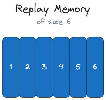
Newer memories kick older ones out, once the size limit of the replay memory is reached. This makes sense since very old memories shouldn't have much impact on what happens now anymore. This also enables the model to adapt to new rules in the game.

Pseudocode
Alright, with this knowledge, let us take a look at the pseudocode from the Playing Atari with Deep Reinforcement Learning paper. The only bits that differ are that they potentially preprocess the state s with some function φ (which we don't do here) and that they remove the max term when the agent reaches a terminal state, i.e., the game ends.

We can now implement this idea in Python!
Implementation
First, let us import some libraries and define some parameters.
import random
from collections import deque, namedtuple

import gymnasium as gym
import numpy as np
import tensorflow as tf
from tqdm.auto import tqdm

n_episodes = 1000 # play 1000 games
eps = 0.4 # exploration rate, probability of choosing random action
eps_decay = 0.95 # eps gets multiplied by this number each epoch...
min_eps = 0.1 # ...until this minimum eps is reached
gamma = 0.95 # discount
max_memory_size = 10000 # size of the replay memory
batch_size = 16 # batch size of the neural network training
min_length = 160 # minimum length of the replay memory for training, before it reached this length, no gradient updates happen
memory_parts = ["state", "action", "next_state", "reward", "done"] # nice names for the part of replay memory, otherweise the names are 0-5
Nothing wild going on here, but please read the comments if something is unclear.
Replay memory
Now, we define the replay, which is only a thin wrapper around a Python deque.
Memory = namedtuple("Memory", memory_parts) # a single entry of the memory replay

class ReplayMemory:
    def __init__(self, max_length=None):
        self.max_length = max_length
        self.memory = deque(maxlen=max_length)

    def store(self, data):
        self.memory.append(data)

    def _sample(self, k):
        return random.sample(self.memory, k)

    def structured_sample(self, k):
        batch = self._sample(k)
        result = {}
        for i, part in enumerate(memory_parts):
            result[part] = np.array([row[i] for row in batch])

        return result

    def __len__(self):
        return len(self.memory)
Here, we defined the memory replay in a way that is easy to use. Let's play around with it before we use it in action. We can do
r = ReplayMemory(max_length=3)

r.store(("a", "b", "c", "e", "f"))
r.store((1, 2, 3, 4, 5))
r.store((6, 7, 8, 9, 0))

print(r.structured_sample(2)) # get 2 random sampples from the replay memory

# Output (for me):
# {
#   'state': array([1, 6]),
#   'action': array([2, 7]),
#   'next_state': array([3, 8]),
#   'reward': array([4, 9]),
#   'done': array([5, 0])
# }
If we add another memory, we will lose the first one:
r.store((0, 0, 0, 0, 0))

print(r.memory)

# Output:
# deque([(1, 2, 3, 4, 5), (6, 7, 8, 9, 0), (0, 0, 0, 0, 0)], maxlen=3)
# no more letters in here!
The model
Let us define a simple model! We will use TensorFlow here, but feel free to use PyTorch, JAX, or whatever.
model = tf.keras.Sequential(
    [
        tf.keras.layers.Dense(16, input_shape=(4,), activation="relu"), # state consists of 4 floats
        tf.keras.layers.Dense(16, activation="relu"),
        tf.keras.layers.Dense(16, activation="relu"),
        tf.keras.layers.Dense(16, activation="relu"),
        tf.keras.layers.Dense(2, activation="linear"), # 2 actions: go left or go right
    ]
)
model.compile(
    loss=tf.keras.losses.MeanSquaredError(),
    optimizer=tf.keras.optimizers.Adam(learning_rate=0.01),
)
Training
With these preparations, let us conduct the training now.
env = gym.make("CartPole-v1")
replay_memory = ReplayMemory(max_length=max_memory_size)

for episode in tqdm(range(n_episodes)): # tqdm makes a nice proress bar
    state, _ = env.reset()
    done = False

    while not done:
        if random.random() < eps:
            action = env.action_space.sample() # random action
        else:
            action = model.predict(state[np.newaxis, :], verbose=False).argmax() # best action according to the model

        next_state, reward, done, _, _ = env.step(action)
        memory = Memory(state, action, next_state, reward, done)
        replay_memory.store(memory)

        if len(replay_memory) >= min_length:
            batch = replay_memory.structured_sample(batch_size) # get samples from the replay memory

            target_batch = batch["reward"] + gamma * model.predict(batch["next_state"], verbose=False).max(axis=1) * (1 - batch["done"]) # R(s, a) + γ·maxₐ N(s') if not a terminal state, otherwise R(s, a)
            targets = model.predict(batch["state"], verbose=False)
            targets[range(batch_size), batch["action"]] = target_batch # set the target for the action that was done and leave the outputs of other 3 actions as they are

            model.fit(batch["state"], targets, verbose=False, batch_size=batch_size) # train for one epoch

        state = next_state

    eps = max(min_eps, eps * eps_decay)
And that's it! It kind of looks like the code for Q-learning, but the simple update of a cell in the table got replaced with one step of gradient descent in the form of a single fit .
Results
The code might run for some hours. You can also log some data during training, such as the reward per episode. Another common practice is to log the model every few episodes, so you don't lose too work much when the training crashes. However, saving models has another benefit: very often, the best model is not the latest one. You can see this when you take a look at my reward plot:

You can see that at first, the agent was quite bad. Around episode 100, the agent got rewards of around 200 already before it dropped again. Around episode 230, the model became exceptional, just to dumb down again until episode 1000, where I ended the training. It is weird, but a common pattern that I also see when other people do reinforcement learning.
Let's play!
What could be better than seeing the model we have trained so painstakingly in action? Right, nothing, so let's get started! First, let us see how a random agent competes.


Wow, the random agent really sucks. The run in the middle looked okay in the beginning, but then the randomness kicked it and prevented the agent from going left. You can recreate sad runs like this via
env = gym.make("CartPole-v1", render_mode="human")

env.reset()
done = False

while not done:
    env.render()
    action = env.action_space.sample()
    _, _, done, _, _ = env.step(action)

env.close()
But you are here for something else, right?
A new challenger appears
Let us load the model of episode 230 to see how it performs in a live test!
model = tf.keras.models.load_model("PATH/TO/MODEL/230") # the model is in my Github, https://github.com/Garve/towards_data_science/blob/main/A%20Tutorial%20on%20Deep%20Q-Learning/230.zip
env = gym.make("CartPole-v1", render_mode="human")

state, _ = env.reset()
done = False
total_reward = 0

while not done and total_reward < 500: # force end the game after 500 time steps because the model is too good!
    env.render()
    action = model.predict(state[np.newaxis, :], verbose=False).argmax(axis=1)[0]
    state, reward, done, _, _ = env.step(action)
    total_reward += reward

env.close()
Well, look at that! The agent can effortlessly balance the pole with minimal movement. However, you can see that it is slightly drifting right, which might be a problem in a long run. Let us increase the artificial restriction of 500 time steps to several thousands and look at a sped-up version:

It seems like the agent is doing fine, even after 500 steps. Awesome!
Conclusion
In this article, we have explained why vanilla Q-learning fails when dealing with large or even potentially infinite observation spaces. Discretized Q-learning can help in this case, but you have to think about how much you discretize to find a balance between the agent's performance and training time.
The discretized Q-learning approach is perfectly fine, but we went for another technique that was successfully applied to learn more complex games — deep Q-learning. Instead of updating entries of a potentially large Q-table, we train a model with a fixed amount of parameters.
Let us be honest though. Deep Q-learning is also a trade-off between training time and agent performance. A small network such as linear regression (no hidden layers) will probably perform horribly. If you have millions of parameters for the cart pole game, it is overkill, and training takes ages.
You have to find a balance as well, it doesn't come for free.
However, judging from the papers, it seems that deep Q-learning is still more promising than discretized Q-learning for more complex games such as Atari games.
Learning from sensory input
So far, we have used the internal state of the environment. In the cart pole game, we were given the position of the car, the speed, angles, and so on. When we, as humans, play games, usually we do not have that luxury. I mean, we couldn't process this information fast enough anyway to be good at the game. We have to rely on visual feedback — the screen — to make quick decisions.
What if the agent could only use the screen output as well? As the authors from the Playing Atari with Deep Reinforcement Learning paper show, it works quite well! As they write:
We apply our method to seven Atari 2600 games from the Arcade Learning Environment, with no adjustment of the architecture or learning algorithm. We find that it outperforms all previous approaches on six of the games and surpasses a human expert on three of them.
The authors use a deep convolutional neural network that takes the screen, processes the image it sees, and outputs the Q-values. To be precise, they don't use a single frame, but the last 4 frames of the game. This allows the model to learn the movement speed and directions of the objects on the screen.
But I will leave it like this for now, we can dive into this topic with a fresh mind in another article!
I hope that you learned something new, interesting, and valuable today. Thanks for reading!
If you have any questions, write me on LinkedIn!
And if you want to dive deeper into the world of algorithms, give my new publication All About Algorithms a try! I'm still searching for writers!