Dynamically Choosing the Right Language Model on Every Query

In this article we'll discuss "LLM routing", an advanced inferencing technique which can automatically choose the right language model, out of a selection of language models, for a given prompt; improving the performance, speed, and cost in LLM-powered systems.

We'll explore four approaches to LLM routing: three from academia and one from industry, in order to form a thorough understanding of the concept and technology. In doing so we'll explore a variety of modeling strategies which are useful in important AI use cases, like self-evaluation, autonomous systems, and decision making in the face of uncertainty.

Who is this useful for? Anyone who wants to forge a deeper understanding of AI, and some of the core approaches necessary to make cutting edge AI powered systems.

How advanced is this post? Earlier sections of this article are accessible to readers of all levels. Later sections are geared more towards data scientists and developers with some level of experience.

Pre-requisites: The earlier sections are accessible to readers of all levels, but later sections have some supporting content which may prove necessary for some less experienced readers.

Disclaimer: During the time of writing, I am not affiliated with unify.ai. All opinions throughout this article are my own and are unsponsored.

A Problem: There Are a Lot of Language Models

Here's a list of 132,781 generative language models (at the time of writing). How do you choose the right one?

One might choose to use whatever most people say the best model is. Maybe GPT-4o, Claude Opus, or Gemini Pro. You can pass all your queries through a big fancy language model and you'll get back state of the art responses. Let's imagine what some of those questions and answers might look like.

User Query: What is the derivative of 3x^32x?
LLM Answer: (3x^32x)(32ln(x)+32)

User Query: what is 2+2?
LLM Answer: 4

User Query: Is water wet?
LLM Answer: The question of whether water is "wet" is a bit of a philosophical and semantic debate rather than a straightforward scientific one. Here's how it breaks down...

Using a best in class, expensive, multi-trillion parameter language model to answer 2+2=4 seems like a waste of resources. The issue is, in many AI powered applications, we have no idea if a user will ask a simple or difficult question. If we want a user to get a good response then we have to assume every query will be difficult, and thus we need to use a big fancy model on even the simplest of queries.

The idea of LLM routing is to analyze queries coming in, and then decide which LLM might be best suited to answer that query.

User Query: What is the derivative of 3x^32x?
Router:     This is a complex query. Let's use GPT-4
GPT-4:      (3x^32x)(32ln(x)+32)

User Query: what is 2+2?
Router:     This is a simple query. Let's use Gemini Nano
Gemini Nano:(3x^32x)(32ln(x)+32)

User Query: Is water wet?
Router:     This is a common question. Let's use GPT-4o
GPT-4o:     The question of whether water is "wet" is a bit of a philosophical and semantic debate rather than a straightforward scientific one. Here's how it breaks down...

The power of LLM routing chiefly comes into play when one wants to reduce cost while maintaining performance. There are a lot of different papers and products exploring the idea of LLM Routing in different ways. Let's start with AutoMix.

AutoMix and the LLM Cascade

Before we discuss AutoMix, I invite you to think about how you might solve an LLM routing problem. Let's say you have three models: Claude Haiku, Sonnet, and Opus, each with very different cost to performance tradeoffs.

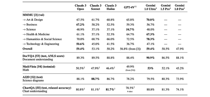
Imagine you were tasked to build a system that could answer incoming queries correctly while minimizing cost. What approach would you take?

Your first intuition might be to develop something called a "LLM cascade" which is exactly what is proposed in both the FrugalGPT and AutoMix papers.

In an LLM cascade you pass a query to the least expensive LLM you have, then ask that same model if the query was answered adequately. If the small model judged that it's own answer was correct, then you return the answer from the small model to the user. If the small model's answer was not deemed correct, you try the same process with a larger model.

This approach can be practical because smaller models can be much, much less expensive than larger models.

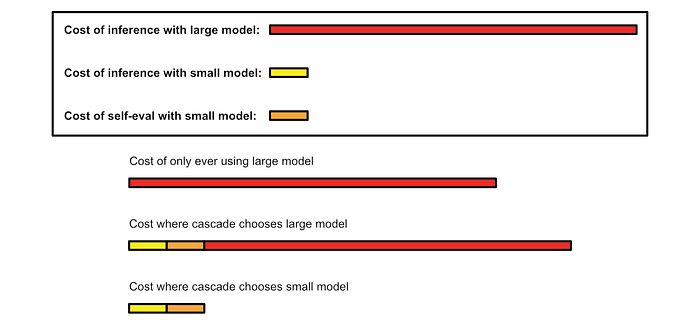
Naturally, an LLM cascade is very dependent on both the users queries and the models chosen, which is where the simplicity of the approach can be a tremendous asset. Because there is no training involved it's incredibly easy to set up and modify a cascade at will.

If you can whip this up in 5 minutes and see a 10x reduction in LLM inference cost with negligible performance impact, then that's pretty neat. However, an issue with this simple approach is that you are likely to see a significant performance drop.

The issue lies in self-evaluation. A lot of the time our smaller language model will be able to tell if it got the answer wrong, but sometimes the smaller model won't be able to detect its own mistakes.

Because LLM cascades rely on self-evaluations to decide whether to continue to a larger model or return the current response, a poor self-evaluation can significantly inhibit the quality of the final output. AutoMix employs something called a "Partially Observable Markov Decision Process" based on "Kernel Density Estimation" to alleviate this problem. Let's unpack those ideas:

A High-Level Intro to POMDPs

A "Partially Observable Markov Decision Process" (POMDP) is an extension of something called a "Markov Decision Process" (MDP).

A Markov Decision Process (MDP) is a way of modeling the types of states a system can be in, and the actions that system can take to transition between states. Say you have a robot, for instance, and you want to allow that robot to navigate through an environment.

You can construct a graph of the possible states that robot can occupy, as well as the cost to transition between states.

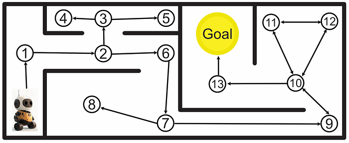
Once the graph is set up, you can analyze that graph to calculate the best course of action.

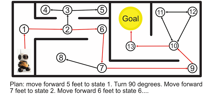
This is called a "Markov Decision Process", and is a super powerful tool in modeling complex systems.

One problem with a classic Markov Decision Process is instability. Imagine we tell our robot to follow the plan to reach the goal, and then the robot's wheel slips halfway down a hallway; resulting in the robot turning slightly. If we continue executing our pre-defined instructions as before, the robot will get stuck in a corner rather than reach its destination.

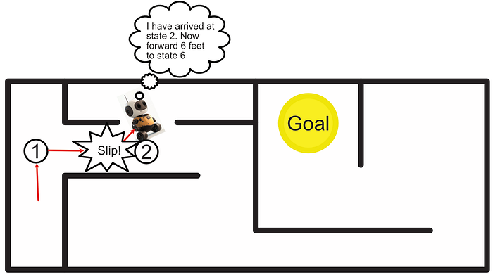
"Partially Observable" Markov Decision Processes (POMDP) are designed to alleviate this problem. The idea of a POMDP is that we assume we never know the true state of the robot, but rather we can make observations and form a probabilistic belief about the state of the system.

If we slap some sensors on our robot, and have it navigate our environment, we can use our sensors to check if we think the robot has ended up in the correct spot. The sensor might not be able to perfectly identify where we are, but we can use our best guess to make a reasonable decision.

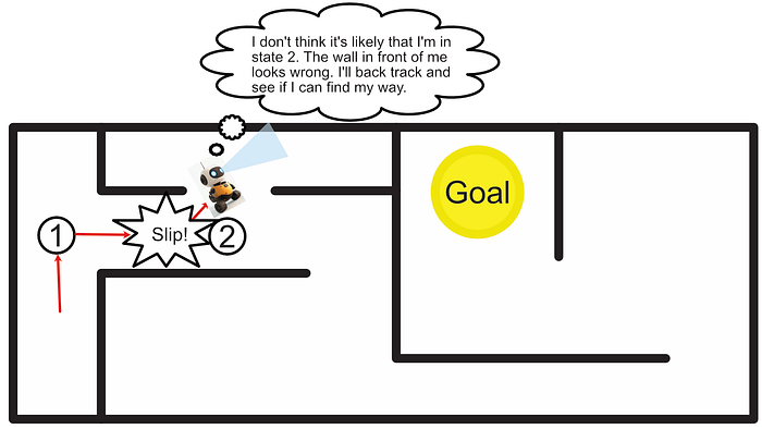
Let's explore how AutoMix employs POMDP's to support the LLM Cascade. In doing so, we'll explore some of the inner workings of POMDP's more in depth.

AutoMix's POMDP Supported LLM Cascade

Full Code for the AutoMix Portion of this article can be found here:

Recall that an LLM Cascade uses self evaluation to either return the response from a smaller language model or pass the prompt to a larger model.

The main idea of AutoMix is, instead of taking the self-evaluations of a model at face value, we turn them into a probabilistic "observation" which hints at the performance of the LLM, then we use that probabilistic observation to decide what action we should take.

To turn a binary "yes or no" self-evaluation into a probability, the authors of AutoMix ask the language models to self-evaluate numerous times with a high temperature setting. Temperature increases how erratic a language models responses are by allowing an LLM to accept output that is occasionally less optimal. If we choose a very high temperature rating, and ask the model to self-evaluate a few times, it allows us to build a probability distribution of self evaluation based on how many times the model says the answer was acceptable or not.

First, we can use langChain's with_structured_output to get a binary true or false evaluation for if an LLM thinks the answer is correct.

"""Creating an "evaluator" using langchain's "with_structured_output".
Basically, this function defines a class which represents the data we want from
the LLM (SelfEval), then langchain uses that class to format the LLMs response into a true
or false judgement of if the model was accurate or not. This allows us to ask an LLM if an
answer was correct or not, and then get back a boolean.

I also have the model form a rationale, before constructing the boolean, serving as a form of
chain of thought.

we specify a high temperature, meaning using an evaluator multiple times
can result in a distribution of evaluations due to high model randomness
"""

from typing import TypedDict
from langchain_openai import ChatOpenAI
from langchain_core.prompts import ChatPromptTemplate

def create_evaluator(model):

    #Defines the structure of the output
    class SelfEval(TypedDict):
        rationale: str
        judgement: bool

    #The system prompt provided to the model
    #prompt lightly modified from AutoMix paper
    self_eval_prompt = ChatPromptTemplate.from_messages(
        [
            (
                "system",
                """Instruction: Your task is to evaluate if the AI Generated Answer is correct or incorrect based on the
provided context and question. Provide ultimate reasoning that a human would be satisfied with, then choose between
Correct (True) or Incorrect (False).
                """,
            ),
            ("placeholder", "{messages}"),
        ]
    )

    #creating a lang chang that outputs structured output
    evaluator = self_eval_prompt | ChatOpenAI(
        model=model, temperature=1 #setting a high temperature
    ).with_structured_output(SelfEval)

    return evaluator

Then we can have a model answer some question

"""Having an LLM answer a riddle

There was a plane crash in which every single person was killed.
Yet there were 12 survivors. How?
"""

from openai import OpenAI

model = 'gpt-3.5-turbo'

context = """There was a plane crash in which every single person was killed. Yet there were 12 survivors. How?"""
question = "Solve the riddle"

client = OpenAI(api_key=api_key)
response = client.chat.completions.create(
        model=model,
        messages=[
            {"role": "user", "content": f"context:\n{context}\n\nquestion:\n{question}"}
            ],
    )

answer = response.choices[0].message.content.strip()

We can use the evaluator we defined to ask the model to evaluate it's own answer a few times, and construct a normal distribution based on how many true and false self evaluations there were.

""" Constructing a normal distribution (a.k.a. bell curve, a.k.a gaussian),
based on 40 self evaluations, showing how likely an answer was right or
wrong based on several LLM self-evaluations.

Gaussians have two parameters:
- the mean, or center of the distribution: calculated as just the average value
- the standard deviation: which is how spread out the values are.

The funciton `gaussianize_answer` runs self eval some number of times,
gets a distribution of self evaluations saying the response was good
or poor, then constructs a gaussian describing that overall distribution.
"""

import numpy as np
import matplotlib.pyplot as plt
from scipy.stats import norm

def gaussianize_answer(context, question, answer):
    num_evaluations = 40
    evaluations = []
    evaluator = create_evaluator(model)

    for _ in range(num_evaluations):

        for i in range(2):
            #allowing the evaluator to make several attempts at judgements
            #and wrapping it in a try/catch to deal with the odd parsing error.
            try:
                evaluation = evaluator.invoke({"messages": [("user", f"""Context: {context}
            Question: {question}
            AI Generated Answer: {answer}""")]})

                evaluations.append(evaluation['judgement'])
                break
            except KeyboardInterrupt as e:
                raise e
            except:
                print('evaluator error')
        else:
            print('too many errors, skipping evaluation step')

    # Calculate probability (mean) of evaluations
    probability = sum(evaluations) / len(evaluations)

    # Calculating mean and standard deviation, which define a gaussian
    mean = probability
    std_dev = np.sqrt(probability * (1 - probability) / len(evaluations))

    return mean, std_dev

mean, std_dev = gaussianize_answer(context, question, answer)

#cant draw gaussian if there's perfect consensus
if mean != 0 and mean !=1:
    # Create a range for x values
    x = np.linspace(0, 1, 100)
    y = norm.pdf(x, mean, std_dev)

    # Plot the Gaussian
    plt.plot(x, y, label=f'Gaussian Distribution\nMean={mean:.2f}, Std Dev={std_dev:.2f}')
    plt.title("Gaussian Distribution of True Value Probability")
    plt.xlabel("Probability")
    plt.ylabel("Density")
    plt.legend()
    plt.show()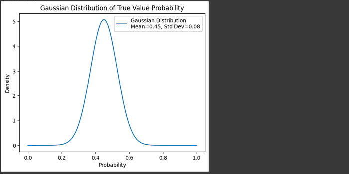

Without using a POMDP, one could simply apply a threshold to these probabilities and use them to make decisions about how to navigate through the cascade, possibly seeing an improvement over using individual self evaluation results. However, self evaluations are know to be noisy and unreliable. Let's do some self-evaluations on several answers and overlay the distributions of correct and incorrect answers to explore just how noisy self-evaluation can be:

"""Creating normal distributions based on self evaluations for a few answers.
Recall that the riddle was the following:

There was a plane crash in which every single person was killed. Yet there were 12 survivors. How?
"""

#A selection of a few hardcoded LLM answers
llm_answers = []
#correct
llm_answers.append("The 12 survivors were married couples.")
llm_answers.append("The people on the plane were all couples - husbands and wives.")
llm_answers.append("The answer to this riddle is that the 12 survivors were married couples.")

#incorrect 
llm_answers.append("The riddle is referring to the survivors being the 12 months of the year.")
llm_answers.append("The riddle is referring to the survivors as the numbers on a clock (numbers 1-12). So, the answer is that the \"12 survivors\" are actually the numbers on a clock.")

#evaluating all answers
distributions = []
for llm_answer in llm_answers:
    mean, std = gaussianize_answer(context, question, llm_answer)
    distributions.append((mean, std))

Here, the first three answers are correct answers to the riddle, while the final two answers are incorrect answers to the riddle. We can plot these distributions to see how well our auto-evaluation strategy can separate good and bad answers.

"""Plotting the gaussians we created in the previous code block.
Correct answers are dotted, wrong answers are solid.
"""

fig = plt.figure(figsize=(10, 6))

#plotting all gaussians
for i, dist in enumerate(distributions):
    #unpacking tuple
    mean, std = dist

    name = f'LLM answer {i}'

    #labeling the two clearly wrong answers as dotted lines (i=3 and i=4)
    if i>=3:
        stroke = '-'
    else:
        stroke=':'

    if std == 0:
        plt.plot([mean,mean],[0,1], linestyle=stroke, label=name)
    else:
        # Create a range for x values
        x = np.linspace(0, 1, 100)
        y = norm.pdf(x, mean, std)
        plt.plot(x, y, linestyle=stroke, label=name, alpha=0.5)
plt.title("Gaussian Distribution of True Value Probability Across Answers")
plt.xlabel("Probability")
plt.ylabel("Density")
plt.legend()
plt.show()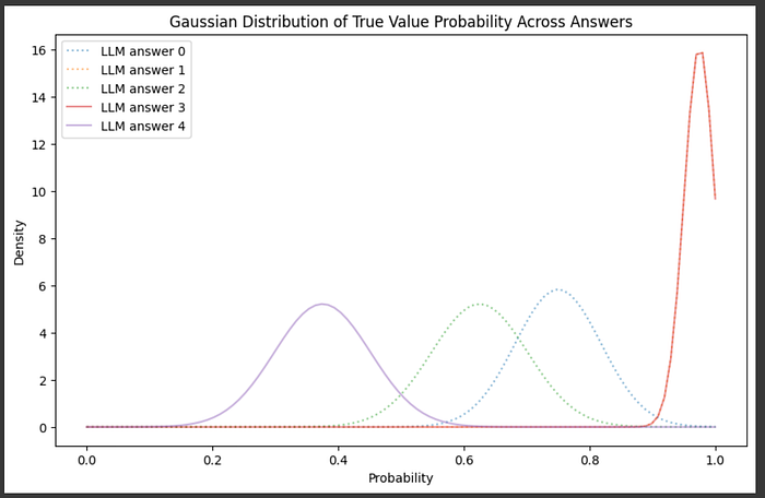

And… It did a pretty bad job. The distributions for good and bad answers are all mixed up. Language models are frustratingly bad at knowing if their own answers are wrong or not. If we use this self-evaluation strategy as-is, our LLM cascade will likely make wrong decisions; sometimes triggering expensive models when it shouldn't and sometimes returning bad responses when it shouldn't.

This is where the "partially observable" aspect of POMDPs comes in. Instead of assuming the self-evaluations we're constructing are accurate, we can treat it like an observation and use that observation to try to predict if an answer is really good or not.

In the AutoMix paper they do that through a process called Kernel Density Estimation (KDE). Say you have a model, and you have a handful of examples where you know the model answered the question correctly and incorrectly. You can do self-eval on question-answer pairs to figure out where self-evaluations typically end up when the models answer is actually correct or incorrect.

In other words, we're going to build a dataset of self-evaluation scores where we know the model's answer is right, and another set where we know the models answer is wrong, then we're going to use that data to make routing decisions.

Here I'm constructing a synthetic dataset of self-evaluations for correct and incorrect answers, but you might imagine running the gaussianize_answer function we previously defined on a bunch of questions and answers to create this dataset.

import numpy as np
import matplotlib.pyplot as plt
import pandas as pd
import seaborn as sns

# Creating a synthetic dataset with self evaluation results
# and actual performance results.
np.random.seed(0)

n_each = 50

selfeval_bad = np.random.normal(0.55, 0.05, n_each)    # Lower confidence around 0.4
selfeval_good_1 = np.random.normal(0.9, 0.03, n_each)  # Higher confidence around 0.7
selfeval_good_2 = np.random.normal(0.6, 0.03, n_each)  # Higher confidence around 0.6
selfeval_good = np.concatenate([selfeval_good_1, selfeval_good_2]) #combining both good distributions
self_eval = np.concatenate([selfeval_good_1, selfeval_good_2, selfeval_bad])
true_performance = [1] * (n_each*2) + [0] * n_each

#plotting a swarm plot
df = pd.DataFrame()
df['true_performance'] = true_performance
df['self_eval'] = self_eval

ax = sns.swarmplot(x="true_performance", y="self_eval", data=df)
plt.title("Training Dataset with True Performance vs Self Evaluation")

plt.show()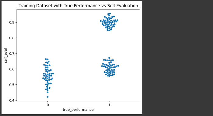

The idea of kernel density estimation (KDE) is to turn these individual examples into smooth density distributions such that we can use them to calculate the probability of a truly good answer. In other words, we want to be able to say "I know self-eval said there was a 50% chance the answer is good, but based on a dataset of self-evaluations I know that almost certainly means the answer is wrong because bad answers at a self evaluation of 0.5 are way more dense than good answers at 0.5". KDEs allow us to do that.

To construct a KDE you first put a gaussian (a.k.a. kernel, a.k.a bell curve) on every point in a distribution:

"""Placing a gaussian with an average value equal to every point
in the distribution of self evaluation results for good predictions
The standard deviation can be modified as necessary. Here I'm defining the
standard deviation as 0.05 for all gaussians, but they could be larger
or smaller, resulting in smoother or more sensitive KDEs
"""

import matplotlib.gridspec as gridspec
from scipy.stats import norm

fig = plt.figure(figsize=(10, 6))

# Creating a gaussian distribution with a small deviation on every point in a set of data
gs = gridspec.GridSpec(2, 1, height_ratios=[2, 1])
ax1 = fig.add_subplot(gs[0])
std = 0.05
for mean in selfeval_good:
    x = np.linspace(0, 1, 100)
    y = norm.pdf(x, mean, std)
    plt.plot(x,y)
plt.xlim([0, 1])
plt.xlabel("Gaussians built on good evaluations")

ax2 = fig.add_subplot(gs[1])
sns.swarmplot(x = 'self_eval', data = df[df['true_performance']==1])
plt.xlim([0, 1])
plt.xlabel("Individual good self evaluations")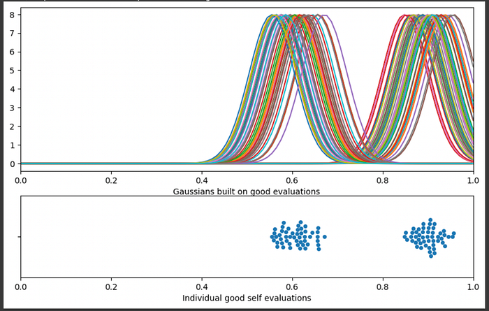

Then we can add them all up to create a smooth volume of predictions. The more predictions there are in a region, the larger the volume is.

"""modifying the code of the previous code block. Instead of saving
many gaussians, each gaussian is added to the same vector of values
In other words, wer're stacking all the gaussians on top of eachother
"""

import matplotlib.gridspec as gridspec
fig = plt.figure(figsize=(10, 6))

# Creating a gaussian distribution with a small deviation on every point in a set of data
gs = gridspec.GridSpec(2, 1, height_ratios=[2, 1])
ax1 = fig.add_subplot(gs[0])
std = 0.05
y = np.zeros(100)
for mean in selfeval_good:
    x = np.linspace(0, 1, 100)
    y += norm.pdf(x, mean, std)
plt.plot(x,y)
plt.xlim([0, 1])
plt.xlabel("Sum of all gaussians built on all good evaluations")

ax2 = fig.add_subplot(gs[1])
sns.swarmplot(x = 'self_eval', data = df[df['true_performance']==1])
plt.xlim([0, 1])
plt.xlabel("Individual good self evaluations")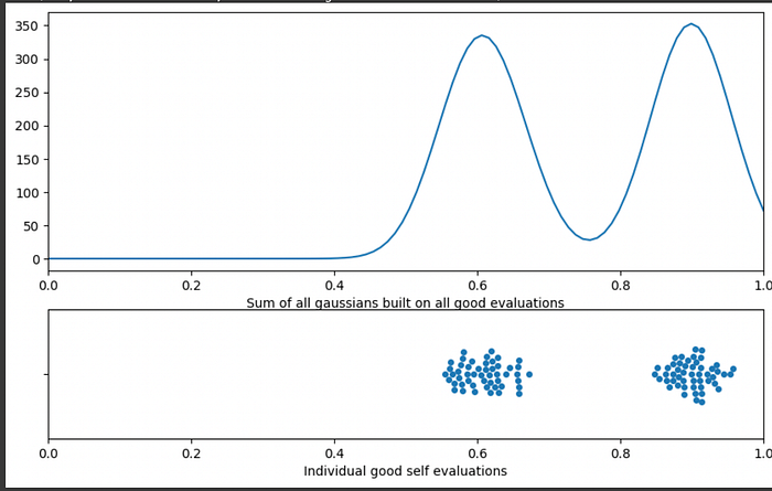

In this graph the y axis doesn't really mean anything. The more data you have, the taller this graph will be, meaning the y axis is dependent on both density and the number of total predictions. Really, we're just interested in density, so we can calculate the area under the curve of the sum of gaussians then divide by that area. That will mean, regardless of how many predictions you have the area under the curve will always be 1, and the height of the curve will be the relative density of one region vs another, rather than being influenced by the number of samples you have.

"""Modification of the previous code block to create a density plot
Calculating the area under the curve, then dividing the values
by that area. This turns a vague volume of results into a density
distribution, essentially getting rid of the impact that larger numbers
of samples tend to make the y axis taller.
"""

import matplotlib.gridspec as gridspec
fig = plt.figure(figsize=(10, 6))

# Creating a gaussian distribution with a small deviation on every point in a set of data
gs = gridspec.GridSpec(2, 1, height_ratios=[2, 1])
ax1 = fig.add_subplot(gs[0])
std = 0.05
y = np.zeros(100)
for mean in selfeval_good:
    x = np.linspace(0, 1, 100)
    y += norm.pdf(x, mean, std)

#converting to density (total area under the curve, regardless of the number
#of samples, will be equal to 1. Densities beteen distributions are comperable even
#if the number of samples are different)
area_under_curve = np.trapz(y, dx=1/100)
y = y/area_under_curve

plt.plot(x,y)
plt.xlim([0, 1])
plt.xlabel("Density of good evaluations")

ax2 = fig.add_subplot(gs[1])
sns.swarmplot(x = 'self_eval', data = df[df['true_performance']==1])
plt.xlim([0, 1])
plt.xlabel("Individual good self evaluations")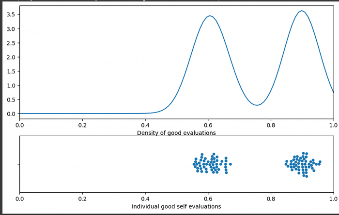

And thus we've constructed a KDE. I know I've been throwing terms around like crazy , so I want to take a moment to reiterate what this graph represents.

We start with a bunch of answers to questions by an LLM, and we get each of those dots in the graph above by asking the LLM to self evaluate a few times with a high temperature on the same question and answer, turning each answer into a probability. Self-evaluations are often noisy and inconsistent, so what we would like to do is find what self-evaluation scores are the most likely to actually correspond to a correct answer. To do that, we're looking at the self-evaluation scores of actually good answers, and finding the region in which self-evaluation scores are more dense. If we have a self evaluation score which lies in a region where there is a high density of actual good answers, then it's probably more likely to be a good self-evaluation.

All that code we made to construct the kernel density estimation can be replaced with scipy.stats.gaussian_kde. We can use that function for the self evaluation of both truly good answers and truly bad answers to get an idea of which self-evaluation values are more likely given a good or bad answer.

from scipy.stats import gaussian_kde

# Perform KDE for each performance state
good_kde = gaussian_kde(selfeval_good, bw_method=0.3)
poor_kde = gaussian_kde(selfeval_bad, bw_method=0.3)

# Define a range of confidence scores for visualization
confidence_range = np.linspace(0, 1.0, 200)

# Evaluate KDEs over the range of confidence scores
good_density = good_kde(confidence_range)
poor_density = poor_kde(confidence_range)

# Plot the KDE for each performance state
plt.figure(figsize=(10, 6))
plt.plot(confidence_range, poor_density, label="Density of Self Eval for Poor Results")
plt.plot(confidence_range, good_density, label="Density of Self Eval for Good Results")
plt.title("KDE of Confidence Scores for Good and Poor Performance")
plt.xlabel("Confidence Score Through Self Evaluation")
plt.ylabel("Density of Predictions")
plt.legend()
plt.show()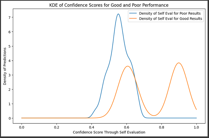

So, if we had a self evaluation of 60%, for instance, we could calculate the probability of if it would actually be a good answer by comparing the relative densities of good and bad answers in that region.

# Plot the KDE for each performance state
plt.figure(figsize=(10, 6))
plt.plot(confidence_range, poor_density, label="Density of Self Eval for Poor Result", alpha=0.7)
plt.plot(confidence_range, good_density, label="Density of Self Eval for Good Result", alpha=0.7)

#plotting the probabilities of good or bad at a given location
sample_confidence = 0.6
conf_poor = poor_kde(sample_confidence)[0]
conf_good =  good_kde(sample_confidence)[0]
label = f'Good Probability: {int(conf_good/(conf_poor+conf_good)*100)}%'
plt.plot([sample_confidence]*3,[0,conf_poor, conf_good], 'r', linewidth=3, label=label)
plt.plot([sample_confidence]*2,[conf_poor, conf_good], 'r', marker='o', markersize=10)

plt.title("KDE of Confidence Scores for Good and Poor Performance States")
plt.xlabel("Confidence Score Through Self Evaluation")
plt.ylabel("Density of Predictions")
plt.legend()
plt.show()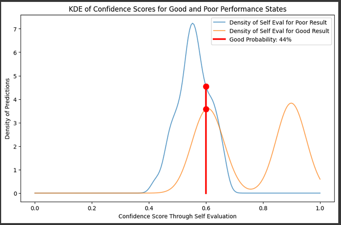

We can sweep through the entire x axis and calculate the probability that an answer is good, based on the ratio of densities of the known training data, across all possible self-evaluation results

plt.figure(figsize=(10, 6))
plt.title("Probability that the prediction is correct based on the difference of the self evaluation distributions")
good_probability = np.array([good/(good+poor) for (good, poor) in zip(good_density, poor_density)])
plt.plot(confidence_range, good_probability)
plt.xlabel("Confidence Score Through Self Evaluation")
plt.ylabel("Probability Correct")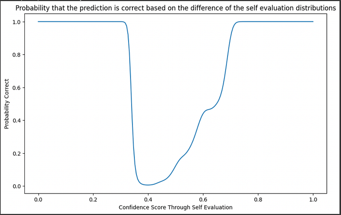

This is pretty nifty, but you might notice a problem. At a self-evaluation score of 0.2, for instance, the probability (based on the ratio of densities) is 100% not because there are a lot of examples of good predictions at that point, but because there aren't any samples in that region.

To deal with this, the AutoMix paper also talks about constructing a KDE across all the data, and only keeping results that have self-evaluations that lie within dense regions of the dataset.

"""Creating a graph of probability that an answer is right
and also a graph of the density of all the training data
"""

import matplotlib.gridspec as gridspec
fig = plt.figure(figsize=(10, 6))

total_kde = gaussian_kde(self_eval, bw_method=0.3)
total_density = total_kde(confidence_range)
height_normalized_total_density = total_density/max(total_density)
confidence_threshold = 0.5
density_threshold = 0.1

#marking 
gs = gridspec.GridSpec(2, 1, height_ratios=[2, 1])
ax1 = fig.add_subplot(gs[0])
plt.plot(confidence_range, good_probability)
threshold = 0.5
plt.fill_between(confidence_range, good_probability, 0, where=(good_probability > confidence_threshold), color='blue', alpha=0.2, label=f'Probability based on density ratios > {confidence_threshold}')
plt.ylabel("Probability Correct")
plt.legend()

ax2 = fig.add_subplot(gs[1])
plt.plot(confidence_range, height_normalized_total_density, label="Normalized density of all self evaluations", alpha=1)
plt.fill_between(confidence_range, height_normalized_total_density, 0, where=(height_normalized_total_density > density_threshold), color='blue', alpha=0.2, label=f'Total normalized density > {density_threshold}')
plt.xlabel("Confidence Score Through Self Evaluation")
plt.ylabel("Density of Predictions")
plt.legend()
plt.show()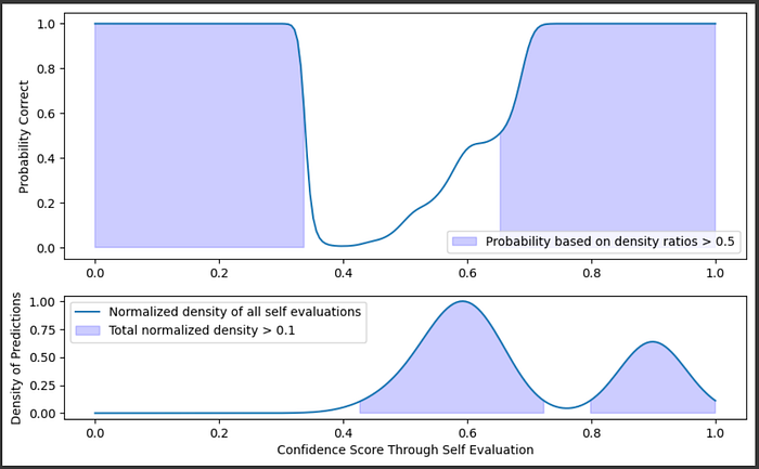

So, we can say a self-evaluation is good if the probability of a prediction is good and if the self evaluation exists within a region where there is a fair amount of training data. Even though the probability might be high at 0.2, we know there's no data at that point, so we would be skeptical of that self-evaluation.

With LLMs, there is generally a tradeoff between cost and performance. We might be willing to accept different probabilities that an answer is good depending on the cost and performance constraints of our use case. We can balance cost and performance by changing the threshold at which we decide to call the larger LLM given a smaller LLM's self-evaluation.

"""Rendering a gradient of cost/performance tradeoff over the graphs
"""

import matplotlib.gridspec as gridspec
fig = plt.figure(figsize=(10, 6))

total_kde = gaussian_kde(self_eval, bw_method=0.3)
total_density = total_kde(confidence_range)
height_normalized_total_density = total_density/max(total_density)
confidence_threshold = 0.5
density_threshold = 0.1

cost_based_thresholds = [0.0,0.1,0.2,0.3,0.4,0.5,0.6,0.7,0.8,0.9]

#marking 
gs = gridspec.GridSpec(2, 1, height_ratios=[2, 1])
ax1 = fig.add_subplot(gs[0])
plt.plot(confidence_range, good_probability)
threshold = 0.5

threshold = cost_based_thresholds[0]
plt.fill_between(confidence_range, good_probability, 0, where=(np.logical_and(good_probability > threshold, height_normalized_total_density > density_threshold)), color='red', alpha=0.2, label=f'bound by cost')

for threshold in cost_based_thresholds[1:-2]:
    plt.fill_between(confidence_range, good_probability, 0, where=(np.logical_and(good_probability > threshold, height_normalized_total_density > density_threshold)), color='red', alpha=0.2)

threshold = cost_based_thresholds[-1]
plt.fill_between(confidence_range, good_probability, 0, where=(np.logical_and(good_probability > threshold, height_normalized_total_density > density_threshold)), color='red', alpha=1, label=f'bound by performance')

plt.ylabel("Probability Correct")
plt.legend()

ax2 = fig.add_subplot(gs[1])
plt.plot(confidence_range, height_normalized_total_density, label="Normalized density of all self evaluations", alpha=1)
for threshold in cost_based_thresholds:
    plt.fill_between(confidence_range, height_normalized_total_density, 0, where=(np.logical_and(good_probability > threshold, height_normalized_total_density > density_threshold)), color='red', alpha=0.2)
plt.xlabel("Confidence Score Through Self Evaluation")
plt.ylabel("Density of Predictions")
plt.legend()
plt.show()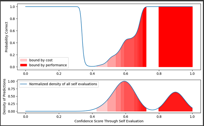

So, based on training data we created of self-evaluations, paired with annotations of if the answers that were self-evaluated were good or bad, we can build a probability distribution of if the answer is actually good or bad, and have a degree of confidence based on the density of our training data within that region. We can use this data to make decisions, thus allowing us to make "observations" about what we think our true performance likely is.

I'll be skipping some fairly verbose code. Feel free to check out the full code:

Imagine we have three LLMS with different abilities to self-evaluate.

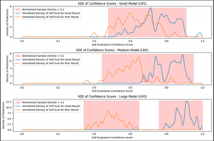
Based on this data, you could use this information to say "I have __% confidence that this answer is actually correct, based on a comparison of a given self evaluation with a dataset of self-evaluations on answers of known quality."

We can feed a query to our tiniest model, have it self-evaluate, and decide if the self evaluation is good enough based on our KDEs for that model. If it's not, we can move onto a bigger model. We do that until we're happy with our output.

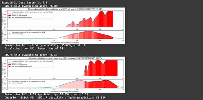
You might notice text about "reward" and "cost" in that output. In LLM routing there's a fundamental tradeoff between performance and cost. If you want better performance it'll be more expensive. If you want lower cost you need to deal with less performance. AutoMix uses the parameter λ (lambda) to control that tradeoff.

We want to consistently achieve high performance at a low cost, but are willing to balance between the two based on λ. If we care more about performance we might use a small λ value, and if we care more about cost we might choose a large λ value. This tradeoff is defined in the reward function:

This can actually get pretty complicated. Formally, in a POMDP we need to account for all probabilities and all costs of all models when making a decision. I'm planning on tackling POMDPs more in depth at some point in the future, and this article has taken long enough to come out, so I simply made the reward function equal to the probability of the current output being good minus λ times the cost of the next model. So, instead of looking at all possibilities of all future models, I'm simply saying "is the current output good enough vs the cost to try again with the next model, based on λ".

Again, full code can be found here.

"""Constructing the POMDP and running it with simulated inferences
This is a simplification of the POMDP which just looks at the probability
of the current self evaluation and the cost of the next model.
"""
class Model:
    def __init__(self, name, kde_good, kde_poor, kde_density, good_threshold, cost):
        """
        Initialize each model with KDEs for good/poor predictions, a good_threshold for trusting its output,
        and a cost associated with using this model.
        """
        self.name = name
        self.kde_good = kde_good
        self.kde_poor = kde_poor
        self.kde_density = kde_density
        self.good_threshold = good_threshold
        self.cost = cost

    def evaluate(self, self_eval, density_threshold=0.2):
        """Calculate the probability that the prediction is good based on the self evaluation score."""
        prob_good = observe_good_probability(self_eval, self.kde_good, self.kde_poor, self.kde_density, 
                                             normalized_density_threshold=density_threshold, model_name=self.name, plot=True)
        plt.show()
        return prob_good


class POMDP:
    def __init__(self, models, lambda_param=0.1):
        """
        Initialize the POMDP with a list of models and the lambda parameter that balances performance vs. cost.
        """
        self.models = models
        self.lambda_param = lambda_param  # Parameter to balance cost vs. performance in reward function

    def compute_reward(self, prob_good, cost):
        """
        Compute the reward based on the performance (prob_good) and the cost of the model.
        """
        return prob_good - self.lambda_param * cost

    def run_simulation(self, n_examples=5):
        """Run the POMDP decision process across multiple examples."""
        for example in range(n_examples):
            print(f"Example {example + 1}. Cost factor is {self.lambda_param}:")
            for model_iter, model in enumerate(self.models):
                self_eval = np.random.uniform(0.6, 1.0)  # Generate a random self-evaluation score
                print(f"  {model.name}'s self-evaluation score: {self_eval:.2f}")
                prob_good = model.evaluate(self_eval)

                # Compute reward based on the current model's performance and cost
                if model_iter<len(self.models)-1:
                    reward = self.compute_reward(prob_good, self.models[model_iter+1].cost)
                    print(f"  Reward for {model.name}: {reward:.2f} (probability good: {prob_good*100:.2f}%, cost of next: {self.models[model_iter+1].cost})")
                else:
                    reward = 1 #no more models to escelate to

                # Decision: Should we trust this model or escalate?
                if reward > 0:  # If the reward is positive, we trust the model
                    print(f"  Decision: Stick with {model.name}. Probability of good prediction: {prob_good*100:.2f}%\n")
                    break  # Stop traversing as we trust this model
                else:
                    print(f"  Escalating from {model.name}. Reward was {reward:.2f}\n")
            else:
                print("  No suitable model found, escalating failed.\n")


# Define models dynamically with their respective KDEs, thresholds, and costs
lm1 = Model("LM1", kde_good_lm1, kde_poor_lm1, kde_density_lm1, good_threshold=0.8, cost=1)
lm2 = Model("LM2", kde_good_lm2, kde_poor_lm2, kde_density_lm2, good_threshold=0.85, cost=1.2)
lm3 = Model("LM3", kde_good_lm3, kde_poor_lm3, kde_density_lm3, good_threshold=0.9, cost=1.5)

# Initialize the POMDP with the list of models and the lambda parameter (balancing performance vs cost)
pomdp = POMDP(models=[lm1, lm2, lm3], lambda_param=0.5)

# Run the simulation
pomdp.run_simulation(n_examples=5)

And here's a few examples of it in action:

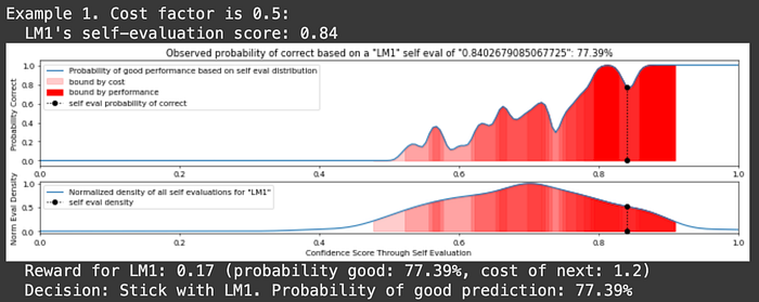
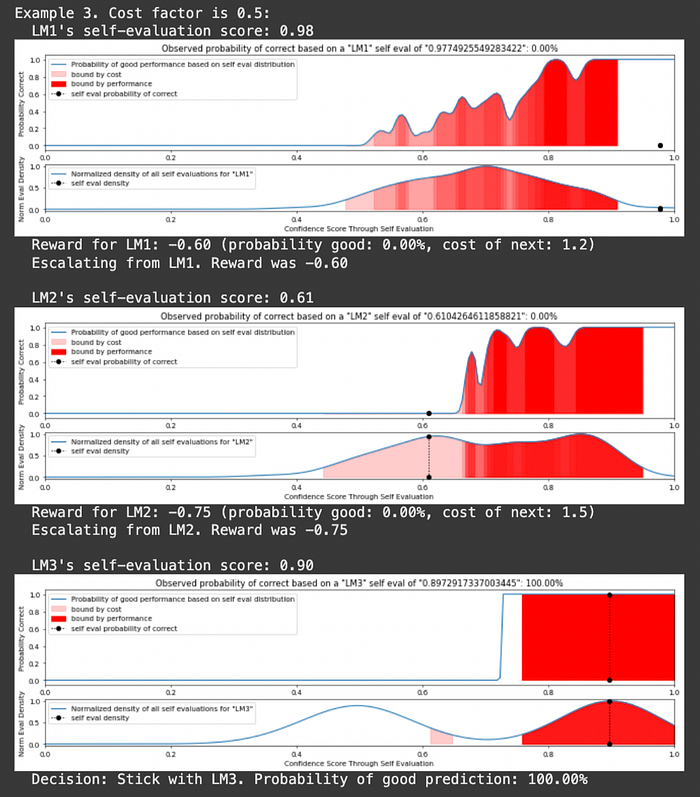
And, ta-da, we have made an AutoMix style POMDP that allows us to balance cost and performance tradeoffs by routing to different LLMs in a cascade. Let's check out a different example of LLM Routing which approaches the problem in a few different ways.

A Few Approaches from RouteLLM

The Route LLM paper presents a few compelling approaches to LLM Routing:

• Similarity Weight Ranking
• Matrix Factorization
• BERT Classification
• Causal LLM Classification

We're going to focus on Similarity Weight Ranking and BERT Classification in this article, but before we dive in I'd like to talk about how RouteLLM differs from AutoMix in terms of the data it uses.

RouteLLM: A Different Approach to Data

The AutoMix approach we discussed previously focuses on being able to whip up an LLM router with very little data. With only a few tens, or perhaps hundreds, of examples of questions and answers you can use that data to build out density estimations and develop AutoMix. This is incredibly powerful because, starting from just a few LLMs and a dream, you can create all the data necessary to build AutoMix by yourself in an afternoon.

RouteLLM takes a much more "big data" approach to LLM Routing by building sophisticated models which make intricate routing decisions. This is a double-edged sword: You might end up with heightened performance, but at an additional cost to get things set up.

Instead of looking at self-evaluation results, like what is done in AutoMix, RouteLLM analyzes the query itself and attempts to make decisions based on which models are better at certain types of queries. To make this more nuanced assessment, they use a ton of data. Specifically:

• The bulk of the data used in RouteLLM is 80k examples of human preference data from chatbot arena, which allows humans to rank the relative performance of two random LLMs with one another on a given query.
• They use the multiple choice dataset MMLU to automatically evaluate if a model was correct or incorrect, with a high degree of certainty, on a given prompt
• The Nectar dataset contains GPT-4's ranking of several smaller models responses.

The data pre-processing of RouteLLM is a fascinating topic, which we'll briefly discuss before getting into how they actually create routers.

Code for the RouteLLM exploration is available here:

Turning Sparse Preference Data into Routing Data

The primary dataset used in the RouteLLM paper is from "Chatbot Arena". Chatbot arena allows users to ask a question to multiple chatbots and rate which one they find to be the best answer to the query. The RouteLLM paper uses this to train a model for routing.

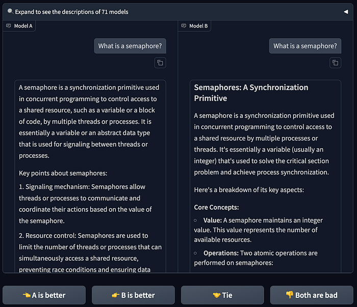
Data from these comparisons is made available on the lmsys/lmsys-arena-human-preference-55k dataset, which tabulates approximately 55 thousand of these comparisons.

One problem with this dataset is label sparsity. If we look at how often each model appears in the dataset, it's pretty infrequent.

"""Getting the 55k dataset and showing how often a particular model appears
as model a
"""
import pandas as pd

df = pd.read_csv("hf://datasets/lmsys/lmsys-arena-human-preference-55k/train.csv")
df['model_a'].value_counts(normalize = True)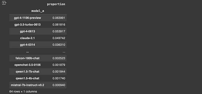

Thus, it's very hard to make a sophisticated model that can route to this or that model specifically, because we don't have a lot of data on each specific model.

To get around this issue, the authors of RouteLLM chose to use an approach called "Elo Scoring". Elo scoring is a popular approach in ranking players in games which have head-to-head competitions, like Chess. If you have several examples where playerA wins & PlayerB looses , PlayerC wins & PlayerB looses , PlayerC wins & PlayerD looses , you can use Elo Scoring to create a score for each player, and thus rank the players from worst to best.

To implement Elo Ranking in this context, you might give each model a default score of 1000, then iterate through all the comparisons in the dataset.

Any time one model wins over another model, you might increase the score of the winning model and decrease the score of the losing model. In Elo Ranking, the magnitude of the score change has to do with the difference between the score of the two models: If one model is much better than another model and wins, then the scores ought not to change much because it was obvious that a much higher ranked model should win. However, if a model with a low score wins against a model with a high score, the change in ranking ought to be more significant as that result implies their scores are very wrong. Typically, there's also a limit to the magnitude of the score change, so scores don't deviate wildly based on lucky victories.

Here I'm implementing Elo Ranking on the chatbot arena dataset to rank the LLMs in order of performance.

"""Iterating through human comparisons and adjusting scores
in order to rank which models are better or worse based on human eval
"""

# Initialize the ELO ratings for each model
elo_ratings = {}

def get_elo(model):
    """Get the ELO rating for a model, defaulting to 1000."""
    return elo_ratings.get(model, 1000)

def update_elo(winner, loser, k=32, draw=False):
    """Update ELO ratings for a winner and loser model, or in case of a draw."""
    winner_elo = get_elo(winner)
    loser_elo = get_elo(loser)

    # Calculate expected scores
    expected_winner = 1 / (1 + 10 ** ((loser_elo - winner_elo) / 400))
    expected_loser = 1 / (1 + 10 ** ((winner_elo - loser_elo) / 400))

    # Define the score outcome
    if draw:
        winner_score = loser_score = 0.5
    else:
        winner_score = 1
        loser_score = 0

    # Update ratings
    elo_ratings[winner] = winner_elo + k * (winner_score - expected_winner)
    elo_ratings[loser] = loser_elo + k * (loser_score - expected_loser)

# Process each row in the DataFrame to update the ELO ratings
for _, row in df.iterrows():
    model_a = row['model_a']
    model_b = row['model_b']

    if row['winner_model_a'] == 1:
        update_elo(model_a, model_b)
    elif row['winner_model_b'] == 1:
        update_elo(model_b, model_a)
    elif row['winner_tie'] == 1:
        update_elo(model_a, model_b, draw=True)

# Convert ELO ratings to a DataFrame for easy viewing
elo_df = pd.DataFrame(list(elo_ratings.items()), columns=['Model', 'ELO Rating']).sort_values(by='ELO Rating', ascending=False)
elo_df.reset_index(drop=True, inplace=True)

# Display the DataFrame using tabulate for a cleaner output
elo_df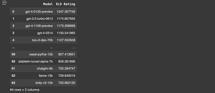

The reason we're bothering to calculate Elo scores is to allow us to group models into "weak" and "strong" categories. Instead of routing to a particular model, the goal of RouteLLM is to decide that a model should be sent to a stronger but more expensive model, or a weaker but less expensive model. Thus, we can train off of groups of these models rather than routing to an individual model, mitigating the problem of label sparsity.

Here is an example of how one might create a group of strong and weak models:

#strong models
strong_models = elo_df[elo_df.Group <=1]['Model'].unique()
strong_models

# weaker than very strong models
weak_models = elo_df[(elo_df.Group>1) & (elo_df.Group<=3)]['Model'].unique()

weak_models

This is not all the data that the RouteLLM team used, they also constructed similar data from other sources, but for our purposes this is the gist of it. Now that we have the data, let's explore how RouteLLM approached routing!

RouteLLM — Similarity Matching with a Bradley-Terry Model

The RouteLLM paper actually explores four different approaches to LLM Routing. We'll only be discussing two: "Similarity Matching with a Bradley-Terry Model" and "BERT Classification"

The idea of "Similarity Matching with a Bradley-Terry Model" is somewhat similar to the approach we discussed previously in AutoMix, in that the Bradley-Terry model is a lightweight modeling strategy which can be executed on the fly. The difference from AutoMix is that this approach uses more data to make decisions, and uses embeddings (rather than self-evaluation in a cascade) to make routing decisions.

If that made sense to you, great. If not, that's ok. In the following sections we'll unpack how Similarity Matching with a Bradley-Terry Model works.

An Overview of the Approach

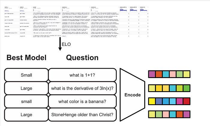
The whole idea of similarity matching hinges on the use of a type of model called an encoder. An encoder takes some arbitrary text and distills it into a numerical representation which somehow represents the text's meaning.

Encoders are popularly used in approaches like "Retrieval Augmented Generation" Which uses the results from an encoder to find which information is similar to other information.

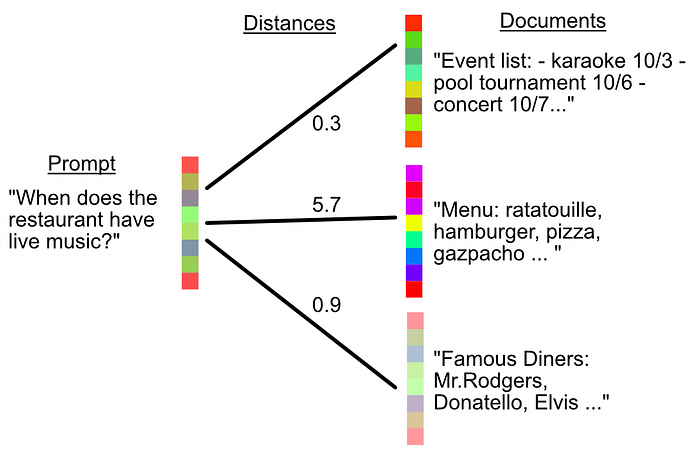
The idea, in the context of routing, is to look through all our question examples and calculate an embedding.

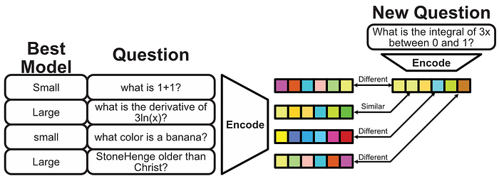
Then, when a new question comes in, we compare how close the embedding is to the questions in our dataset.

We can then use the closeness of the embeddings to decide if a small or large model is more appropriate.

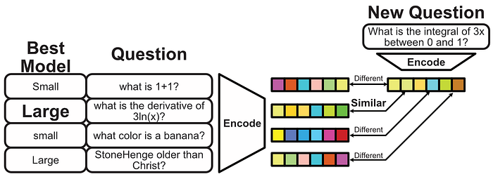
Of course, we could pretty much stop there. If more of the similar questions require a large model, then use a large model. The Authors of AutoMix decided to go with a slightly more sophisticated approach called a Bradley-Terry model.

The Bradley-Terry Model

I'll likely be covering Bradley-Terry models and their applications in a dedicated article sometime soon. For now, we can cover the idea from a high level.

Essentially, a Bradley-Terry model is a lightweight model that can be rapidly trained to make a prediction between a pairwise comparison. It can take many forms, but the most naive and simplistic form is this:

Essentially, we can say how likely two mutually exclusive things are to happen (thing i vs thing j) if we know the probabilities of thing i happening and thing j happening.

This is cool but it isn't really a model, it's just a function. The Bradley-Terry Model comes into play when we add in a few parameters.

This is useful because if we know the probability of "thing i vs thing j" happening (think the probability that we need a big vs a small model), then we can learn the parameters βi and βj that work best across numerous examples.

The AutoMix paper chooses to use a slightly different form, which is essentially equivalent, and swaps out the symbol ξ for β

The important thing to know now is that this equation has parameters which we can learn to allow the Bradley-Terry model to output a probability of something happening. So, if we know the probability firsthand (how probable it is that a large model should be chosen, which we know as 100% or 0% based on human preference data) we can learn parameters ξwi and ξli to build a model that can learn to output that probability.

If this doesn't make complete sense, don't worry, we'll wash over it a few times in the following sections.

An Overview of AutoMix's Use of The Bradley-Terry Model

From AutoMixe's prospective, we know the probability that a given query should use a large or small model. We know this because we've grouped models into large and small categories, and have the humans preferences.

So, when we get a new query, the idea is to find the queries in the dataset which are the most similar, use those similar queries to train a Bradley-Terry(B-T) model, and then use that Bradley-Terry model to make a prediction as to weather the new query should use a small or large model.

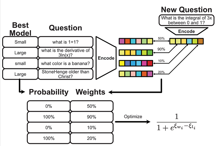
This approach is more sophisticated than just saying "this query is similar, so we should use the same size model", because it allows us to make adjustments based on the proximity of the new query to many queries in the dataset. We can use "kind of similar" queries to update our model "a little bit", and "more similar queries" to update our model "more".

The way they did that in the AutoMix paper is by turning proximity to the query into a weight, then using those weights to dictate how much a given example in our dataset can impact the training of the Bradley-Terry(B-T) model.

Let's work through and implement this approach with code.

Implementing AutoMix's Bradley-Terry Model

Again, full code can be found here.

First, recall that we previously calculated which models were strongest and which models were weakest, and grouped them into two groups. Let's first create a dataframe consisting of the prompts and if strong or weak models should be chosen on similar prompts.

# Filter rows where there's a match between a strong and a weak model
matches = df[((df['model_a'].isin(strong_models)) & (df['model_b'].isin(weak_models))) |
             ((df['model_a'].isin(weak_models)) & (df['model_b'].isin(strong_models)))].copy()

# Reconstruct DataFrame to show whether strong or weak model won
def identify_winner(row):
    if row['model_a'] in strong_models and row['winner_model_a'] == 1:
        return 'strong'
    elif row['model_b'] in strong_models and row['winner_model_b'] == 1:
        return 'strong'
    elif row['model_a'] in weak_models and row['winner_model_a'] == 1:
        return 'weak'
    elif row['model_b'] in weak_models and row['winner_model_b'] == 1:
        return 'weak'
    else:
        return 'tie'

# Apply the identify_winner function to create a new column
matches.loc[:, 'Winner'] = matches.apply(identify_winner, axis=1)  # Use .loc to set the new column

# Select and rearrange columns for clarity
result_df = matches[['Winner', 'prompt']]
result_df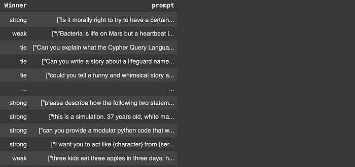

We need to take all the queries in the dataset and calculate embeddings. When we get some new query in the we'll calculate an embedding for it in a similar way.

"""Embedding all 
"""
import numpy as np
import pandas as pd
from langchain.embeddings import OpenAIEmbeddings

# Initialize the LangChain OpenAI embeddings model
embeddings_model = OpenAIEmbeddings(model="text-embedding-ada-002")  # Use the small model

# Get batch embeddings for all prompts in result_df
prompts = result_df['prompt'].tolist()

#sanatizing
prompts = [p.replace('<|endoftext|>', '') for p in prompts]

result_df['prompt_embedding'] = embeddings_model.embed_documents(prompts)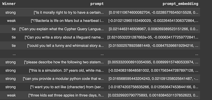

So, we have a big list of embeddings for our training data, and we will have an embedding from a new query. Now let's define a way to calculate similarity.

We do this using cosine similarity, which is the type of "distance" that AI encoders are typically based off of. With cosine similarity, Vectors that are pointing in similar directions are considered close, and vectors pointing in different directions are considered to be far apart.

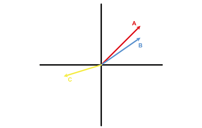
We can calculate the cosine similarity using the following expression:

This doesn't really mean much on its own. We don't care how big or small these numbers are, but rather how big they are relative to each other. I want to know the most similar queries out of all my queries in my dataset, so I can make a routing decision.

Thus, the authors of AutoMix chose to normalize these similarity scores, squashing all values into a range from 0 to 1, where 1 is the closest item.

Then, because researchers love math, they calculate a weight with the following expression:

why? I don't care. This article is like two months late. It's probably practically useful when actually training the Bradley-Terry model. They recommend a value of γ=10. Here's my implementation of weight calculation given an embedding for a new query and a bunch of existing embeddings:

import numpy as np

def calculate_weight(new_query_embedding, training_query_embeddings, gamma=10):
    """Returns a weight for each training query embedding via normalized cosine similarity.
    Parameters:
    - new_query_embedding: numpy array of shape [embedding_dim], the embedding of the new query.
    - training_query_embeddings: numpy array of shape [N, embedding_dim], embeddings of training queries.
    - gamma: float, scaling factor for the weight calculation.
    Returns:
    - weights: numpy array of shape [N], weights for each training query embedding.
    """

    #calculating cosine similarity of the new query vs all training queries
    dot = np.dot(training_query_embeddings, new_query_embedding)
    norms_training = np.linalg.norm(training_query_embeddings, axis=1, keepdims=True)
    norm_new = np.linalg.norm(new_query_embedding)
    cosine_similarities = (dot/(norms_training.T*norm_new))[0]

    #Normalizing cosine similarities by max value
    normalized_similarities = cosine_similarities/max(cosine_similarities)

    #calculating weight
    return gamma ** (1+normalized_similarities)

# Testing with sample data
# Create a random embedding for the new query
np.random.seed(0)
new_query_embedding = np.random.rand(10)

# Create random embeddings for training queries
training_query_embeddings = np.random.rand(10, 10)

# Calculate weights
weights = calculate_weight(new_query_embedding, training_query_embeddings, gamma=10)
weights

Anyway.

We now have a weight for each element in the dataset based on how similar that element is to a new query asked by the user.

Using these weights we can train the Bradley-Terry (B-T) model, which will ultimately be the thing that gives us our routing decision.

To do that, we'll use the following optimization function proposed by the RouteLLM paper.

Let's unpack this element by element.

"argmin" means we want to search for the minimum value of this function by changing the value of ξ (in this case ξwi and ξli)

This function accounts for every element within our table of preference data. We'll tally up some score for all the data in our preference dataset, and attempt to minimize the total score.

For a given preference instance i, we're going to scale the importance by the weight of that instance.

And this is the meat of what we're really minimizing:

The function ℓ is called "binary cross entropy". I don't think we need to get into the weeds, but it's a very common function in data science. If you have something that is supposed to be a 0 or a 1, and a prediction like 0.1 or 0.9, the binary cross entropy function will give you a big number if your prediction is far away from what it should have been, and a small number if it's close.

Here, li is what a particular prediction should have been (we know the router should have predicted for a big or small model because we have the preference data. This might be a 1 or a 0)

and we're comparing that to the output of our Bradley-Terry (B-T)model, which gives us a probability.

In implementing the B-T model, I just had two ξ values: one for if the model should be big, and one for if the model should be small. Then I use those two parameters in the Bradley-Terry (B-T) model to give me a probability. These are initialized as random values in the beginning.

Then I compared the output of the B-T model to what the probability ideally should have been using binary cross entropy, resulting in a loss value we want to minimize

I scaled that loss value by how similar that example in the preference data was to the original query. I then also scaled it by a small learning rate so that each example in the data has only an incremental impact on the parameters.

I then updated the ξ values in the Bradley-Terry (B-T) model to be less wrong, based on this δ value.

If we iterate this process over all the preference, we'll eventually find ξ values which minimize the loss for the B-T model with respect to all the preference data and how similar it is to the user's query.

Here's the code:

def compute_coefficients(weights, labels, learning_rate=0.01, epochs=20):
    """Computes the Bradley-Terry Coefficients based on the weights and labels for each query.

    Parameters:
    - weights: numpy array of shape [N], weights for each training query embedding.
    - labels: numpy array of shape [N], binary labels (0 or 1) for each training example.
    - learning_rate: float, learning rate for gradient descent. This is a small number because
                     we only want to update our parameters a little bit for each example
    - epochs: int, number of iterations for gradient descent.

    Returns:
    - xi: numpy array of shape [2], optimized BT coefficients for small and large models
    """

    def binary_cross_entropy_loss(label, probability):
        """Calculate binary cross-entropy loss for a single example with probability clipping to avoid log(0)."""
        epsilon = 1e-10  # Small value to prevent log(0)
        probability = np.clip(probability, epsilon, 1 - epsilon)
        return -(label * np.log(probability) + (1 - label) * np.log(1 - probability))

    # Initialize coefficients (xi) randomly, one for each class
    # In the RouteLLM paper they learn one coefficient for 10 parititions,
    # But I found the details to be confusing. I'm computing coefficients for
    # small models and large models as we defined previously

    #the labels represent if large is necessary (1) or not (0), so index 0
    #of this should represent the coefficient of the large model not being
    #necessary, and index 1 represents the coefficient large model being
    #necessary. These coefficients will be optimized to bias one vs the other.

    # note: The BT model is optimized for *every query*, meaning
    # these will be optimized based on the similarities weights
    # for an individual case.
    xi = np.random.rand(2)

    #if there's a strong bias towards one model or the other throughout the data,
    #the BT model will learn that bias heavily, and thus won't learn routing nuance.
    #As a result, we're going to balance against that bias by biasing the gradient
    #of the loss when the label indicates a large model. If the large model is
    #called more often in the training, then this value will be <1. If less often,
    #this value will be >1.
    
    #note, this had no appreciable effect so I won't discuss it
    large_model_bias = 1/(labels.sum()/len(labels))


    for epoch in range(epochs):
        total_loss = 0
        gradients = np.zeros_like(xi)

        for i, (weight, label) in enumerate(zip(weights, labels)):
            # Calculate the probability using the Bradley-Terry model
            # this essentially asks the bradley terry model, based on the two
            # coefficients, how likely it is that a large model is necessary (1)
            delta = np.clip(xi[1] - xi[0], -500, 500)  # Clipping to prevent overflow in exp
            probability = 1 / (1 + np.exp(-delta)) #probability of a large model being required

            # Calculate the cross-entropy loss
            loss = binary_cross_entropy_loss(label, probability)
            weighted_loss = weight * loss
            total_loss += weighted_loss

            #Scaling loss if the model is large, according to bias
            if label:
                loss = large_model_bias*loss

            # Calculating gradients
            # Here I'm seperatly defining the direction to push the gradients,
            # based on the label, and the magnitude of that push based on the
            # weight and loss.

            # direction is based on if the prediction should be towards large
            # +1 for towards large, -1 for towards small
            direction = (label*2-1)

            gradient_large = direction*(weight * loss)
            graident_small =(-1*direction)*(weight * loss)

            # xi[0] = small model, and xi[1] = large model
            gradients = np.array([graident_small, gradient_large])

        # it made more sense to me to represent the chang in terms
        # of what should be happening, rather than minimizing loss,
        # so here we're adding the gradients rather than subtracting them
        # this isn't really coacher but it made sense to me
        xi += learning_rate * gradients

        # Optional: Print loss for monitoring
        if epoch % 5 == 0:
            print(f"Epoch {epoch}, Total Loss: {total_loss}")

    return xi

if True:
    # Testing the functions with sample data
    # Create random embeddings for new and training queries
    np.random.seed(10)
    n_classes = 2
    n_examples = 10
    embedding_dim = 20

    new_query_embedding = np.random.rand(embedding_dim)
    training_query_embeddings = np.random.rand(n_examples, embedding_dim)

    # Calculate weights
    weights = calculate_weight(new_query_embedding, training_query_embeddings, gamma=10)

    # Generate random binary, corresponding to if a large is necessary (1) or not (0)
    labels = np.random.randint(0, n_classes, size=n_examples)

    # Compute BT coefficients
    coefficients = compute_coefficients(weights, labels, learning_rate=0.01, epochs=10)
    print("Computed BT coefficients:", coefficients)

And now for the upshot

We can compute these BT coefficients every time a new query comes in. So we're not defining a large routing model, we're using the similarity of a new query to define a new model every time we want to make a routing decision. When we get a new query the embedding will be different, which means the weights will be different, which means the optimization will be different, which means the coefficients will be different, which means the prediction by the BT model will be different.

So, we're training a new, tiny routing model every time we want to decide where a particular query should go. Pretty neat!

The Only Problem

Super cool—I think this approach is really compelling. The only issue is, I couldn't get it to work. I defined some code that iterated through the training data and used the BT model to come up with routing decisions from data in the training set. The BT model failed to make any substantive decisions.

import math

#reformatting the training data
bt_data = result_df[['prompt_embedding', 'Winner']].reset_index(drop=True)
bt_data.loc[:, 'Winner'] = bt_data['Winner'].map({'strong':1, 'weak':0, 'tie':0})

labels = bt_data['Winner'].values
embeddings = np.array(list(bt_data['prompt_embedding'].values))

#defining a function for computing the bradley terry model
#and routing accordingly
def route_with_BT_model(query, embeddings, threshold=0.5):
    """This function essentially does _ things:
    1. it embeds the query
    2. it compares the embedded query to the embedded training data,
    and uses those comparisons to construct a bradley terry model
    3. it uses the bradley terry model (which is essentially just two
    coefficients) to make a prediction of if a large or small model is
    appropriate
    4. it compares that probability with a probability threshold, allowing
    us to control the implicit cost/performance tradeoff of using small and
    large llms

    the threshold essentially says how confident we need to be that a small
    model is sufficient in order to route to it. 0.5 would lean on the BT
    model, <0.5 would be cost saving, and >0.5 would bias for performance.
    """

    #embedding query
    query_embedding = np.array(embeddings_model.embed_documents(query)[0])

    #calculating weights, based on the training datas similarity
    #to the query. gamma=10 is recommended
    weights = calculate_weight(query_embedding, embeddings, gamma=10)

    #optimizing a Bradley-Terry model, based on the weights
    coefficients = compute_coefficients(weights, labels, learning_rate=0.01, epochs=10)

    print('coefficients:')
    print(coefficients)

    #computing probability based on the coefficients
    #the way the data is set up, a value of 1 is routing to large models,
    #and a value of 0 routes to small models.
    prob_large = 1/(1+np.exp(coefficients[0]-coefficients[1]))

    return prob_large

indexes = [0,1,2,3,4,5,6,7]

for i in indexes:
    print('======================')
    s = result_df.iloc[i]
    print(s['Winner'])
    prom_large = route_with_BT_model(s['prompt'], embeddings[:10,:])
    print(f'predicted {prom_large}, should have predicted {round(s["winner_label"])}')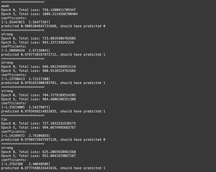

It's entirely possible I messed up some aspect of the implementation, but I decided not to dig further as the result of a test I conducted.

Basically, we have all these fancy "Bradley-Terry optimization based on closeness" shenanigans, but at the end of the day we need to be able to distinguish between queries that have similar or different requirements. Ideally, when we get a query, we want to be able to say "this query is similar to this bunch of queries, and all of these queries require a large model". So, there should be some substantive difference between the embeddings for queries which require a large model, and embeddings which require a small model.

I whipped up a quick function that took a question, and found how close that question was to all other questions in the human evaluated preference data. For this system to work, the embeddings for questions that require the same model should be closer than questions that require a different model. However, in my testing there was no notable distinction.

import matplotlib.pyplot as plt

# Exploring the underlying distance distributions of weak and strong queries
def explore_closness_of_index(result_df, index):
    """finds how close index is to all others
    and returns key metrics
    """

    #getting the partitions being analyzed
    df = result_df.reset_index(drop=True)
    item = df.loc[index]
    df_other = df.drop(index, axis=0)

    #getting the embeddings
    embedding = np.array(item['prompt_embedding'])
    other_embeddings = np.array(list(df_other['prompt_embedding'].values))

    #getting labels of what model should be chosen
    item_label = round(item['winner_label'])
    other_labels = round(df_other['winner_label'])

    #weight, as previously defined, is essentially just cosine similarity normalized,
    #so I can use that to conveniently calculate closeness
    weights = calculate_weight(embedding, embeddings, gamma=1.1)

    # Separate closeness values based on whether they match the target label
    same_label_closenesses = [c for c, l in zip(weights, other_labels) if l == item_label]
    different_label_closenesses = [c for c, l in zip(weights, other_labels) if l != item_label]

    # Plot the overlayed histogram
    plt.figure(figsize=(16, 4), dpi=80)
    plt.hist(same_label_closenesses, bins=15, alpha=0.5, label='Same Label', edgecolor='black', density=True)
    plt.hist(different_label_closenesses, bins=15, alpha=0.5, label='Different Label', edgecolor='black', density=True)

    # Add labels and legend
    plt.xlabel('Closeness')
    plt.ylabel('Frequency')
    plt.title(f'Overlayed Histogram of Closenesses by Label for index {index}')
    plt.legend()

    # Display the plot
    plt.show()

    # return weights

#getting how close a certain question is to other questions that have
#the same or different requierments
explore_closness_of_index(result_df, 0)
explore_closness_of_index(result_df, 1)
explore_closness_of_index(result_df, 2)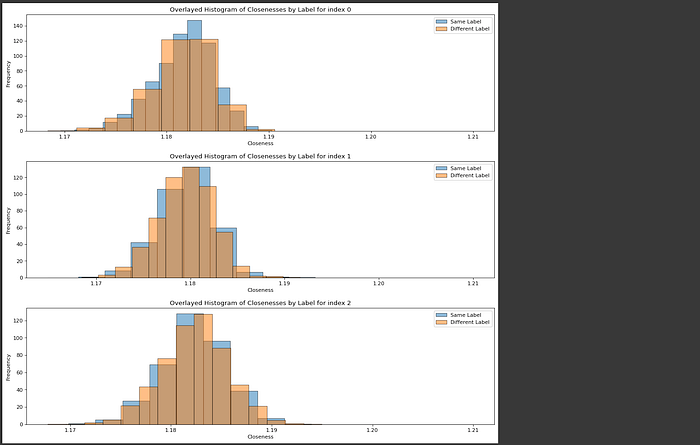

Again, it's entirely possible I messed something up, but I find it very unlikely that a two parameter model could stand any chance at untangling this virtually perfectly overlapped set of distributions.

In my personal opinion, I think this approach relies too much on OpenAI's encoders to embed text as a vector (they used text-embedding-3-small, which I tested in my development). While off-the-shelf encoders are amazing at organizing information, they're not magic. The encoder wasn't trained on organizing queries based on this task specifically. As a result, I personally think it's dubious to expect any simple model that uses an off the shelf encoder to magically be able to perfectly separate data spatially in a way that a Bradley-Terry model could work with.

I do think, however, using a Bradley-Terry model in this fashion, in conjunction with an encoder designed specifically for this task, could be a very compelling approach. I may experiment with that some time in the future, but for now feel free to check out my article on CLIP, which contains a lot of the core ideas around creating encoders.

Let's move into our last major approach, which is mentioned in both RouteLLM and the industrial example we'll be exploring.

LLM Routing With BERT

Before we really get into this approach, I want to briefly cover what a BERT style model is.

A Brief Introduction to BERT

"BERT" stands for Bidirectional Encoder Representations from Transformers. Essentially, it's very similar to a classic transformer like GPT or Claude or whatever, except a bert-style model is designed to understand text rather than generate it.

This change in priorities allows BERT-style models to be trained on different types of data, and also allows BERT to employ subtle modeling tricks which can encourage better comprehension of text. As a result, BERT style models have been very successful in things like classifying if a review was positive or negative, or understanding if certain text should follow other text.

This skill, of knowing if sentence A should follow sentence B, is a big concept for BERT style models, and is called "textual entailment".

am example of the type of textual entailment data BERT is trained on:

Follows | Sentences
------------------
True    | ('I am sad.', 'I ate a bagle, but I'm still hungry')
False   | ('I am sad.', 'I'm not sure if Fudruckers has bagles, though.')
...

We can essentially hijack this skill of BERT style models to do LLM Routing.

The Essential Idea of Routing with BERT

Let's take a quick look at a diagram of a BERT style model. This is from my article on BERT.

There's a lot of stuff going on here that we don't really have to get into for this article. Basically, to train a BERT style model you give it two sentences, like "I am sad" and "I ate a bagel but I'm still hungry", and you pass those into the input of the model. You might occasionally mask out random words, in this case the word "am" is masked, but we don't have to worry about that.

what's important for us is the [CLS] token. This token is a random vector that's passed into the input, and is then passed through the model. After the [CLS] token has passed through the model, it's used to make a prediction of if the two input sentences belong to each other or not. In the diagram above, it's being used to predict that the two sentences do belong together.

The entire idea of the [CLS] token, and really the entire idea of BERT, is to make a model that is forced to intimately understand text and make a classification based on that text. In order for a BERT-style model to be able to say "this sentence follows that sentence", the BERT-style model has to be able to understand sentences. We can then use a BERT-style model's implicit and general-purpose understanding of text and modify the model slightly so it can be applied to a specific task, in oure case LLM Routing.

Both RouteLLM and the example from industry we'll be exploring employ BERT style models. Let's dive into them both:

RouteLLM's approach to BERT-based routing

RouteLLM uses the following expression to describe how they employ a BERT style model:

Basically, they just stuck a neural network onto the [CLS] output of a BERT model, and have that neural network predict which model should be routed to. They then fine tune the entire model, both the BERT style model as well as this tiny neural network, based on the human preference data from chatbot arena.

And… that's it. It's funny, the bigger the models get, the simpler the descriptions often are. Here's the lion's share of what the RouteLLM authors have to say about it, it's only one paragraph:

I have an article on fine-tuning if you want to get a bit more in the weeds on this subject:

Fine tuning is also a fundamental part of the typical training process in BERT style models, which I discuss at length in the BERT article:

BERT-based LLM Routing is also done in the industrial example, which I'd like to discuss next.

BERT Style LLM Routing in Unify.ai

unify.ai is a company run by a professional friend of mine, and he was kind enough to peel back the veil and explain to me how exactly their technology works. Again, this article is not sponsored in any way, I just think it's a cool application of the technology.

unify.ai has two things going for it: it's a central API for talking with a variety of different LLMs, which is cool.

But, more importantly for us, they also have routers that allow you to dynamically choose which LLM you're talking to based on the query.

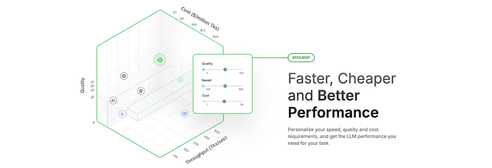
They really think of LLM routing as a give and take between three key constraints:

• Cost: how much will an answer cost
• Quality: how good will your answer be
• Throughput: how quickly will you get your answer

And they essentially allow you to dial in those preferences and get a router between multiple LLMs based on your needs.

Let's discuss how Unify approaches predicting Quality.

Quality Prediction via BERT in Unify.ai

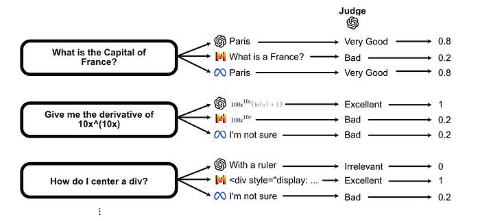
In the Unify implementation of LLM Routing, it starts with a big list of questions.

Each of these questions is then passed to some set of language models to generate answers.

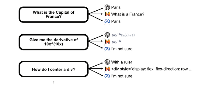
Once each model has created answers based on the dataset of questions provided, they use GPT-4 to judge whether answers to questions were Irrelevant, Bad, Satisfactory, Very Good or Excellent. These are mapped to a 0–1 score for that particular LLM answer.

Under the hood, the list of models gets initialized as a vocabulary of vectors, and then are appended to the query to form the input to the model. Given this input of a model, query pair, the model is tasked with predicting the score. In actually predicting the score, they essentially just put a dense network onto the CLS token.

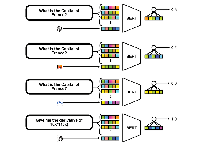
I find this approach of summarizing models as a representative vector to be particularly interesting as it allows the BERT model to compare different LLMs, and how they differ in terms of performance across the same types of questions, throughout the training process. This, in theory, could result in some level of understanding of specific LLMs and how they differ from one another.

Along with constructing BERT-style models for quality prediction, Unify also records real-time metrics in terms of cost-per-token and time-per-token metrics for a variety of models hosted on a variety of cloud services.

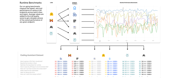
paired with cost per token rates for each of these endpoints, Unify maximizes the following reward function when making a routing decision based on a query:

Where:

• Quality: The quality prediction by the BERT style model, for a given query and model
• ITL: Inter-Token Latency, how long it takes for each token to be generated by the model on average
• TTFT: Time To First Token, the time it takes the first token to be generated. This can be a useful metric in specific use cases which benefit from immediate response, like chat applications
• Cost: The cost of the model to generate a token

When a new query comes in, the Unify router takes into account the predicted quality of each LLM, as well as real time metrics about cost and availability, in order to make routing decisions between both models and endpoints.

Conclusion

In this article we covered four approaches to LLM Routing, all with the same goal: to try to make better LLM powered systems by optimally choosing the right language model to send a given query.

• The first approach featured an LLM cascade supported by kernel density estimations, to give us an idea of how accurate self-evaluations might be based on real data.
• The second approach used textual encoders to try to route based on similarity of a query to a dataset of queries that have known best models based on human preference data. The end routing decision was predicted based on the probability output of a Bradley-Terry model which was optimized against how similar the user's query was to all the data.
• The third approach used the same data as the second approach, but used a BERT-style model to make a classification of if a big or small model should be used based on the query
• The fourth approach also used a BERT-style model, but with a slightly more sophisticated input structure, allowing it to route to specific LLMs. It also accounted for real time metrics, allowing a practitioner to balance performance, cost, and speed.

Join Intuitively and Exhaustively Explained

At IAEE you can find:

• Long form content, like the article you just read
• Thought pieces, based on my experience as a data scientist, engineering director, and entrepreneur
• A discord community focused on learning AI
• Regular Lectures and office hours