The F1 score (aka F-measure) is a popular metric for evaluating the performance of a classification model.

In the case of multi-class classification, we adopt averaging methods for F1 score calculation, resulting in a set of different average scores (macro, weighted, micro) in the classification report.

This article looks at the meaning of these averages, how to calculate them, and which one to choose for reporting.

Contents

(1) Recap of the Basics (Optional) (2) Setting the Motivating Example (3) Macro Average (4) Weighted Average (5) Micro Average (6) Which average should I choose?

(1) Recap of the Basics (Optional)

Note: Skip this section if you are already familiar with the concepts of precision, recall, and F1 score.

Precision

Layman definition: Of all the positive predictions I made, how many of them are truly positive?

Calculation: Number of True Positives (TP) divided by the Total Number of True Positives (TP) and False Positives (FP).

Recall

Layman definition: Of all the actual positive examples out there, how many of them did I correctly predict to be positive?

Calculation: Number of True Positives (TP) divided by the Total Number of True Positives (TP) and False Negatives (FN).

If you compare the formula for precision and recall, you will notice both look similar. The only difference is the second term of the denominator, where it is False Positive for precision but False Negative for recall.

F1 Score

To evaluate model performance comprehensively, we should examine both precision and recall. The F1 score serves as a helpful metric that considers both of them.

Definition: Harmonic mean of precision and recall for a more balanced summarization of model performance.

Calculation:

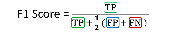
If we express it in terms of True Positive (TP), False Positive (FP), and False Negative (FN), we get this equation:

(2) Setting the Motivating Example

To illustrate the concepts of averaging F1 scores, we will use the following example in the context of this tutorial.

Imagine we have trained an image classification model on a multi-class dataset containing images of three classes: Airplane, Boat, and Car.

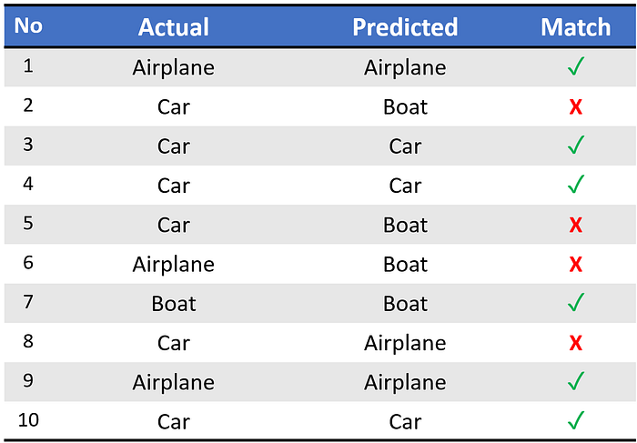
We use this model to predict the classes of ten test set images. Here are the raw predictions:

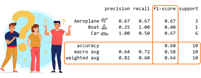
Upon running sklearn.metrics.classification_report, we get the following classification report:

The columns (in orange) with the per-class scores (i.e., score for each class) and average scores are the focus of our discussion.

We can see from the above that the dataset is imbalanced (only one out of ten test set instances is 'Boat'). Thus the proportion of correct matches (aka accuracy) would be ineffective in assessing model performance.

Instead, let us look at the confusion matrix for a holistic understanding of the model predictions.

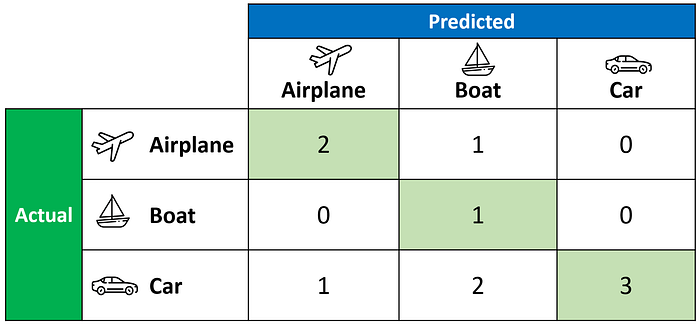
The confusion matrix above allows us to compute the critical values of True Positive (TP), False Positive (FP), and False Negative (FN), as shown below.

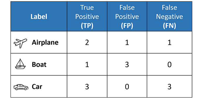
The above table sets us up nicely to compute the per-class values of precision, recall, and F1 score for each of the three classes.

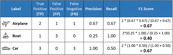
It is important to remember that in multi-class classification, we calculate the F1 score for each class in a One-vs-Rest (OvR) approach instead of a single overall F1 score, as seen in binary classification.

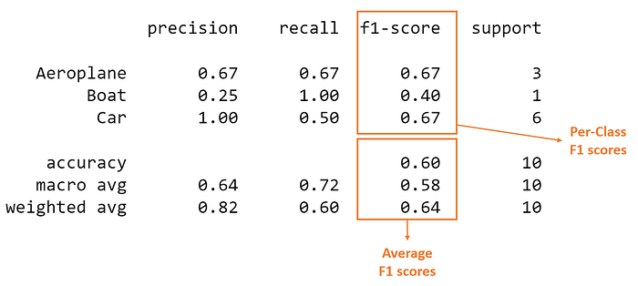
In this OvR approach, we determine the metrics for each class separately, as if there is a different classifier for each class. Here are the per-class metrics (with the F1 score calculation displayed):

However, instead of having multiple per-class F1 scores, it would be better to average them to obtain a single number to describe overall performance.

Now, let's discuss the averaging methods that led to the classification report's three different average F1 scores.

(3) Macro Average

Macro averaging is perhaps the most straightforward among the numerous averaging methods.

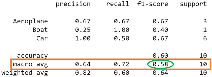
The macro-averaged F1 score (or macro F1 score) is computed using the arithmetic mean (aka unweighted mean) of all the per-class F1 scores.

This method treats all classes equally regardless of their support values.

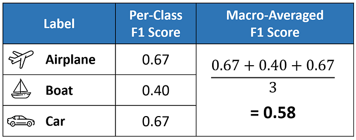
The value of 0.58 we calculated above matches the macro-averaged F1 score in our classification report.

(4) Weighted Average

The weighted-averaged F1 score is calculated by taking the mean of all per-class F1 scores while considering each class's support.

Support refers to the number of actual occurrences of the class in the dataset. For example, the support value of 1 in Boat means that there is only one observation with an actual label of Boat.

The 'weight' essentially refers to the proportion of each class's support relative to the sum of all support values.

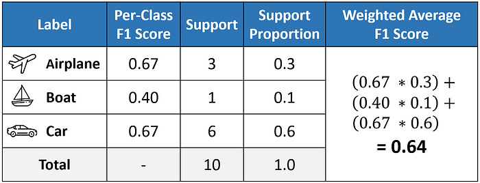
With weighted averaging, the output average would have accounted for the contribution of each class as weighted by the number of examples of that given class.

The calculated value of 0.64 tallies with the weighted-averaged F1 score in our classification report.

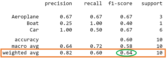
(5) Micro Average

Micro averaging computes a global average F1 score by counting the sums of the True Positives (TP), False Negatives (FN), and False Positives (FP).

We first sum the respective TP, FP, and FN values across all classes and then plug them into the F1 equation to get our micro F1 score.

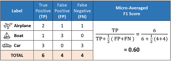
In the classification report, you might be wondering why our micro F1 score of 0.60 is displayed as 'accuracy' and why there is NO row stating 'micro avg'.

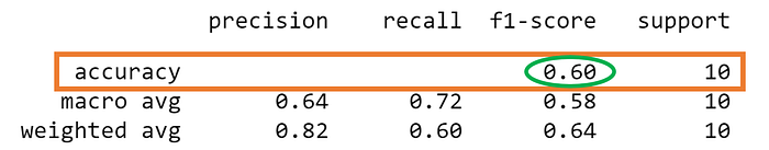
This is because micro-averaging essentially computes the proportion of correctly classified observations out of all observations. If we think about this, this definition is what we use to calculate overall accuracy.

Furthermore, if we were to do micro-averaging for precision and recall, we would get the same value of 0.60.

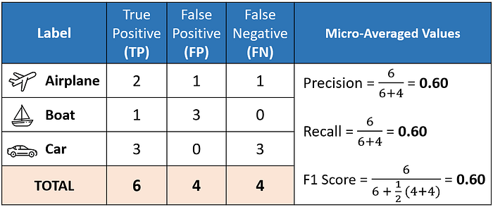
These results mean that in multi-class classification cases where each observation has a single label, the micro-F1, micro-precision, micro-recall, and accuracy share the same value (i.e., 0.60 in this example).

And this explains why the classification report only needs to display a single accuracy value since micro-F1, micro-precision, and micro-recall also have the same value.

micro-F1 = accuracy = micro-precision = micro-recall

(6) Which average should I choose?

In general, if you are working with an imbalanced dataset where all classes are equally important, using the macro average would be a good choice as it treats all classes equally.

It means that for our example involving the classification of airplanes, boats, and cars, we would use the macro-F1 score.

If you have an imbalanced dataset but want to assign greater contribution to classes with more examples in the dataset, then the weighted average is preferred.

This is because, in weighted averaging, the contribution of each class to the F1 average is weighted by its size.

Suppose you have a balanced dataset and want an easily understandable metric for overall performance regardless of the class. In that case, you can go with accuracy, which is essentially our micro F1 score.

Before You Go

I welcome you to join me on a data science learning journey! Follow my Medium page and check out my GitHub to stay in the loop of more exciting data science content. Meanwhile, have fun interpreting F1 scores!