Time series foundation models are finally taking off!

The previous articles explored 2 promising foundation forecasting models, TimeGPT and TimesFM.

This article will explore MOIRAI [1], a groundbreaking TS foundation model by Salesforce. MOIRAI is awesome in terms of performance — but more importantly, the authors have pledged to open-source the model and its training dataset!

This is mentioned in a tweet here by Caiming Xiong, VP of AI at Salesforce and one of the paper's authors

The major contributions of this paper are the following:

• MOIRAI: A novel transformer-encoder architecture, functioning as a universal time-series forecasting model.
• LOTSA (Large Open Time Series Archive): The largest collection of open time series datasets with 27B observations across 9 domains.
• UNITS: An open-source library for training universal time-series models.

Moreover, this article discusses:

1. How MOIRAI works and why it's a powerful model.
2. How MOIRAI performs compared to Google's TimesFM
3. MOIRAI benchmark results.
4. Why MOIRAI will revolutionize the TS forecasting field.

Let's get started.

I've launched AI Horizon Forecast, a newsletter focusing on time-series and innovative AI research. Subscribe here to broaden your horizons!

Challenges of Foundation Time-Series Models

We described the challenges in detail here. To recap, these are:

• Difficulty finding public time-series data — for training a time-series foundation model.
• Time-series data are highly heterogeneous — unlike in NLP, where data have well-defined grammar and vocabulary.
• Time series can be multivariate — unlike in NLP, where input is one-dimensional.
• Time series have different granularities — daily, weekly, monthly, etc.
• Probabilistic forecasting is crucial for decision-making — but each probabilistic model usually optimizes for a specific distribution (arbitrarily).

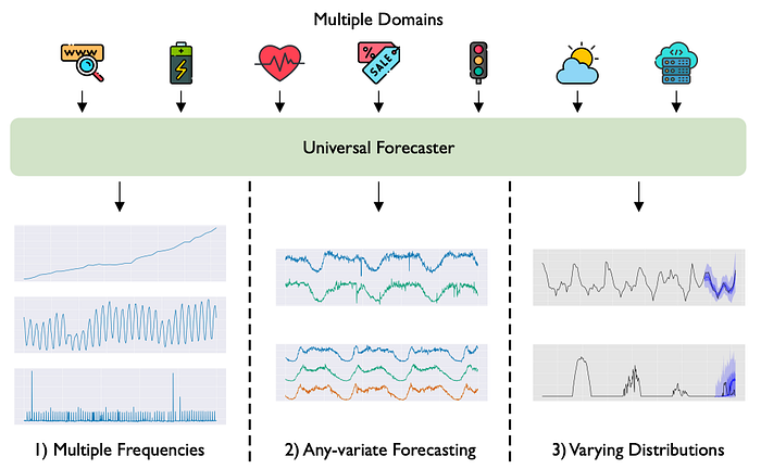
Ideally, a universal TS model should handle the vast heterogeneity of billions of time series. Most importantly, it should accurately zero-shot forecast unseen time series without requiring specific training on them.

Enter MOIRAI

MOIRAI is an encoder-only Transformer model, specialized in universal time-series forecasting.

MOIRAI introduces the following novelties:

• Multi-Patch Layers: MOIRAI adapts to multiple granularities by learning a different patch size for each granularity.
• Any-variate Attention: An elegant attention mechanism that respects permutation variance between each variate, and captures the temporal dynamics between datapoints.
• Mixture of parametric distributions: MOIRAI does not arbitrarily hypothesize a certain distribution. Instead, it optimizes for learning a mixture of distributions.
• Modern LLM features: MOIRAI leverages the latest features of other successful LLMs — ROPE embeddings, SwiGLU activation functions, RMSNorm etc.

Don't worry if you don't understand everything. In the following sections, we'll explain every MOIRAI's feature in detail.

Multi-Patch Layers

Patching is a clever technique where a window of timepoints is transformed and processed as an embedding (like a token in NLP).

Patches were initially introduced in Vision Transformers and became popular in time-series forecasting with PatchTST. Subsequently, they found application in time-series forecasting — notably in Google's TimesFM foundation model.

MOIRAI took this idea further by uniquely using patches: Instead of employing a global patching process for every time series, MOIRAI learns different patch sizes for each frequency. The higher the frequency, the larger the patch size.

Intuitively, this approach is logical: For lower frequency data (e.g. yearly), a larger patch isn't necessary to capture temporal dynamics. Conversely, for high-frequency data, such as data at the second-level, a larger patch size is more suitable. The authors propose the following sizes per frequency:

Note: Interestingly, multi-patching is similar to the mixture-of-experts idea that LLMs have leveraged (like Mixtral) to improve text generation for different formats — code generation, maths calculations etc.

Patching is applied to every variate/covariate. MOIRAI flattens the input, including the covariates — and then patching is applied. This process is visualized in Figure 2 (for patch size=64)

The figure shows a time series where variates 0 and 1 are target variables (i.e. to be forecasted) and variate 2 is a covariate (known in the future):

1. First, the target variables and the covariate are flattened to a single vector.
2. Given a patch size of 64, each variate is patchified into 3 tokens/embeddings.
3. The shaded parts of variates 0 and 1 represent the parts that should be forecasted, hence they are masked. Variate 2 is known in the future, so it remains unmasked.
4. The patched embeddings, along with the variate id and the time id are then passed to the Transformer blocks.
5. MOIRAI's any-variate attention is then calculated — more to that later.
6. Finally, the output patch layer calculates the output.

Now, pay attention to the following:

• In total, we have 2 patch layers.
• The input patch layer is just a linear layer — mapping a window of datapoints to a patch embedding.
• The output patch layer is also a linear layer — mapping a vector to distribution parameters.
• Remember, MOIRAI is probabilistic — the model predicts the parameters of a mixture of distributions. This is similar to what e.g. DeepAR does, by estimating the parameters μ and σ of a normal distribution, which is used to generate the forecasts. However, MOIRAI estimates multiple distributions.
• MOIRAI learns one linear layer per patch size, sharing weights across all examples. For a dataset with 3 frequencies, MOIRAI learns 3 input projection layers and 3 output projection layers. For the LOTSA dataset, MOIRAI learns 5 input and 5 output projection layers for 5 patch sizes: 8, 16, 32,64, and 128 (as shown in Figure 1).

Any-Variate Attention

Perhaps the biggest breakthrough of MOIRAI is the Any-Variate Attention, a novel mechanism with the following advantages:

• Preserves the permutation invariance among different covariates.
• Captures the temporal information among datapoints.
• Accommodates any number of variates.

To achieve this, MOIRAI uses rotary positional embeddings (ROPE) to capture time dependencies, and binary attention biases to capture dependencies among variates.

But first, let's provide some context about self-attention and its significance for time-series:

Why self-attention is permutation-invariant

Given a sentence, attention calculates the relative importance of each word compared to every other word — as pairwise scores.

Consider the sentence "music inspires emotion". Figure 3(top) shows the full-attention matrix weights, where a<i,j> is the attention between words at positions i and j.

Now, let's permute the words to create the sentence "emotion inspires music". Since attention is calculated as pairwise scores between words, we can also permute the respective attention weights (Figure 3 bottom):

While the 2 sentences have different meanings, their permutation leads to the same attention scores — hence attention is permutation invariant.

In NLP, this is acceptable — as attention aims to find the context of a word within a sentence. Additionally, we can apply extra positional embeddings to encode position.

This suffices for textual tasks but falls short for time-series, where sequential ordering is crucial. That's why initial attempts to apply a Transformer (using vanilla attention and naive absolute position encodings) didn't work as expected.

The Elegance of Any-Variate Attention

Now that things are clear, an attention mechanism for time-series should achieve the following:

1. No permutation invariance for the temporal information — the ordering of datapoints should matter.
2. Permutation invariance between the variates/features — ordering of the variates should not matter (e.g. if we have 2 covariates X1 and X2, it does not matter which is first, just the relationship between them).

The attention score between the (i,m)-th query and the (j,n)-th key, where i,j represent the time indexes and (m,n) the variate indexes, is calculated as follows:

E_<ijmn> = E_<time-index-of-query, variate-index-of-query, time-index-of-key, variate-index-of-key>

Embeddings x are multiplied with W_Q or W_K to calculate the query and key vectors respectively. The attention score is calculated by multiplying each query vector with every other key — except there is no value here.

Consider the example of Figure 5. Vector A and vector B belong to the same variate, while Vector C belongs to a different variate. The plot shows the attention score indexes between VectorA — VectorB and VectorA — VectorC:

Consequently, Any-Variate Attention captures the temporal dependencies with precision — while distinguishing between different variates and allowing any number of variates.

The attention formula also includes a rotation matrix R.

The choice of ROPE embeddings is also pivotal here. Instead of using absolute positional embeddings (e.g. in the original Transformer) or relative embeddings (e.g. in T5), ROPE embeddings (via the rotation matrix R) capture the relative distance of two tokens/vectors via their angle, while also maintaining information about their absolute position.

Mixture of parametric distributions

MOIRAI was also developed for probabilistic forecasting.

In neural network-based architectures, there are 2 popular approaches to integrate probabilistic forecasting within a model:

1. Predicting multiple heads (as quantiles) — and then minimizing a quantile loss function.
2. Estimating the parameters of a probability distribution by minimizing the log likelihood loss.

MOIRAI adopts the second approach. This method also offers the advantage of making the model agnostic to specific error metrics like MAE or MASE.

The problem is to determine which probability distribution MOIRAI should optimize for. An obvious choice is the normal distribution. But imagine if the task is sales predictions — where the predictions cannot take any negative values.

As MOIRAI functions as a foundation model, it should adapt to every forecasting task. To achieve this, the model learns the parameters of a mixture of distributions:

• A Student's t-distribution, serving as a general forecaster.
• A log-normal distribution for right-skewed data, commonly encountered in financial and natural phenomena.
• A negative binomial distribution for positive data.
• A low variance normal distribution for high-confidence predictions.

You can find more about the parameters of these distributions in the original paper.

Training

An important contribution of this paper is the LOTSA dataset, which consists of 27B observations and spans 9 domains (Figure 6):

Also, the authors trained 3 MOIRAI models, of sizes 14M, 91M, and 311M parameters. Their characteristics are shown in Figure 7:

The larger model was trained for 10⁶ steps with a batch size of 256 on NVIDIA A100–40G GPUs.

It is worth mentioning the context and prediction lengths that the model used for training.

Since MOIRAI is a universal model and should adapt to every context and prediction length, the authors trained the model on multiple context and prediction lengths for each time series. Therefore, the training process involved data augmentation — meaning the model was actually trained on more than 27 billion instances.

Benchmark Results

The authors evaluated MOIRAI in 2 scenarios:

• In-distribution forecasting: The model was fine-tuned on a portion of the training data.
• Out-of-distribution forecasting(zero-shot): The model performs zero-shot forecasts on unseen datasets — against other SOTA models specifically trained on those datasets.

In the first scenario, the Monash repository was used as an evaluation dataset. The authors used the normalized MAE (by normalizing using the MAE of the naive model)(Figure 8)

In the zero-shot scenario, the authors used the Continuous Ranked Probability Score (CRPS) and Mean Scaled Interval Score (MSIS) — suitable for probabilistic forecasting. Moreover, MOIRAI was tested against llmtime, another zero-shot foundation model that uses GPT-3.5 and LLaMA-2 as base models (Figure 9):

We notice the following:

• In the in-distribution setting, MOIRAI is the clear winner.
• In the zero-shot setting, MOIRAI (especially the large version) is the best (or second-best) in most datasets.
• Interestingly, the base version also achieves top positions in some datasets.
• Remember, in the 2nd scenario, MOIRAI does zero-shot inference — meaning that MOIRAI had never seen that data during training — contrary to the other models.

Comparison with TimesFM

TimesFM is also a revolutionary foundation model that was released recently.

Both models use similar ideas (patching, transformer blocks, etc). The main differences are:

• TimesFM is a decoder-style Transformer, while MOIRAI mostly resembles an encoder-based architecture.
• MOIRAI uses multiple patches to accommodate different frequencies, while TimesFM supports one type of patching.
• The largest MOIRAI has more parameters (311M) compared to TimesFM(200M). On the other hand, TimesFM seems to be trained on more data compared to TimesFM (100B vs 27B).
• MOIRAI uses a more refined attention mechanism compared to TimesFM. Also, the decision for MOIRAI to use a mixture of probability distributions is ingenious.
• Both models demonstrate strong zero-shot performance. MOIRAI also provides extra details regarding the effect of in-distribution forecasting (TimesFM does not).
• In terms of raw performance, we can't be sure which model comes first. Even if TimesFM was also open-source, it's not clear what data exactly has seen during training.

Criticism MOIRAI does not provide any details regarding how the model scales in terms of parameter size, data, and training time. Remember, the potential of a large Transformer-based model depends on its ability to leverage scaling laws.

TimesFM does not provide specific details either — but at least its authors show it becomes better with more data.

Closing Remarks

MOIRAI is a foundation time-series model that will revolutionize time-series forecasting.

It's also a modern model, leveraging many features from other successful LLMs like Meta's LLaMA models.

In addition to the model itself, releasing a large open-source dataset is a significant milestone — it will speed up research in large-scale forecasting and serve as a platform for future benchmarks!

Thank you for reading!

• Follow me on Linkedin!
• Subscribe to my newsletter, AI Horizon Forecast!
• Check some cool time-series projects!

References

[1] Woo et al., Unified Training of Universal Time Series Forecasting Transformers (February 2024)