Why should you read this post?
The training/inference processes of deep learning models are involved lots of steps. The faster each experiment iteration is, the more we can optimize the whole model prediction performance given limited time and resources. I collected and organized several PyTorch tricks and tips to maximize the efficiency of memory usage and minimize the run time. To better leverage these tips, we also need to understand how and why they work.
I start by providing a full list and a combined code snipped in case you'd like to jump into optimizing your scripts. Then I dive into them one by one in detail afterward. For each tip, I also provide code snippets and annotate whether it's specific to the device types (CPU/GPU) or model types.
Checklist:
- Data Loading
1. Move the active data to the SSD
2.
Dataloader(dataset,num_workers=4*num_GPU)3.Dataloader(dataset,pin_memory=True) - Data Operations
4. Directly create vectors/matrices/tensors as
torch.Tensorand at the device where they will run operations 5. Avoid unnecessary data transfer between CPU and GPU 6. Usetorch.from_numpy(numpy_array)ortorch.as_tensor(others)7. Usetensor.to(non_blocking=True)when it's applicable to overlap data transfers 8. Fuse the pointwise (elementwise) operations into a single kernel by PyTorch JIT - Model Architecture 9. Set the sizes of all different architecture designs as the multiples of 8 (for FP16 of mixed precision)
- Training
10. Set the batch size as the multiples of 8 and maximize GPU memory usage
11. Use mixed precision for forward pass (but not backward pass)
12. Set gradients to
None(e.g.,model.zero_grad(set_to_none=True)) before the optimizer updates the weights 13. Gradient accumulation: update weights for every other x batch to mimic the larger batch size - Inference/Validation 14. Turn off gradient calculation
- CNN (Convolutional Neural Network) specific
15.
torch.backends.cudnn.benchmark = True16. Use channels_last memory format for 4D NCHW Tensors 17. Turn off bias for convolutional layers that are right before batch normalization - Distributed optimizations
18. Use
DistributedDataParallelinstead ofDataParallel
Code snippet combining the tips No. 7, 11, 12, 13:
# Combining the tips No.7, 11, 12, 13: nonblocking, AMP, setting
# gradients as None, and larger effective batch size
model.train()
# Reset the gradients to None
optimizer.zero_grad(set_to_none=True)
scaler = GradScaler()
for i, (features, target) in enumerate(dataloader):
    # these two calls are nonblocking and overlapping
    features = features.to('cuda:0', non_blocking=True)
    target = target.to('cuda:0', non_blocking=True)
    # Forward pass with mixed precision
    with torch.cuda.amp.autocast(): # autocast as a context manager
        output = model(features)
        loss = criterion(output, target)
    # Backward pass without mixed precision
    # It's not recommended to use mixed precision for backward pass
    # Because we need more precise loss
    scaler.scale(loss).backward()
    # Only update weights every other 2 iterations
    # Effective batch size is doubled
    if (i+1) % 2 == 0 or (i+1) == len(dataloader):
        # scaler.step() first unscales the gradients .
        # If these gradients contain infs or NaNs,
        # optimizer.step() is skipped.
        scaler.step(optimizer)
        # If optimizer.step() was skipped,
        # scaling factor is reduced by the backoff_factor
        # in GradScaler()
        scaler.update()
        # Reset the gradients to None
        optimizer.zero_grad(set_to_none=True)
High-level concepts
Overall, you can optimize the time and memory usage by 3 key points. First, reduce the i/o (input/output) as much as possible so that the model pipeline is bound to the calculations (math-limited or math-bound) instead of bound to i/o (bandwidth-limited or memory-bound). This way, we can leverage GPUs and their specialization to accelerate those computations. Second, overlap the processes as much as possible to save time. Third, maximize the memory usage efficiency to save memory. Then saving memory may enable a larger batch size, which saves more time. Having more time facilitates a faster model development cycle and leads to better model performance.
1. Move active data to SSD
Some machines have different hard drives like HHD and SSD. It's recommended to move the data, which will be used in the active projects, to the SSD (or the hard drive with better i/o) for faster speed.
#CPU #GPU #SaveTime
2. Asynchronous data loading and augmentation
num_workers=0 would make data loading execute only after training or previous process is done. Setting num_workers >0 is expected to accelerate the process more especially for the i/o and augmentation of large data. For GPU specifically, this experiment found that num_workers = 4*num_GPU had the best performance. That being said, you can also test the best num_workers for your machine. To be noted, high num_workers would have a large memory consumption overhead (ref), which is also expected, because more data copies are being processed in the memory at the same time.
Dataloader(dataset, num_workers=4*num_GPU)#CPU #GPU #SaveTime
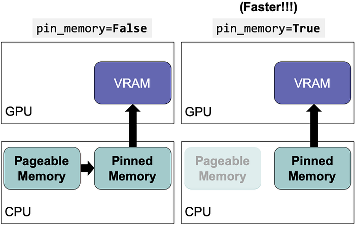
3. Use pinned memory to reduce data transfer

GPU cannot access data directly from the pageable memory of the CPU. The setting, pin_memory=True can allocate the staging memory for the data on the CPU host directly and save the time of transferring data from pageable memory to staging memory (i.e., pinned memory a.k.a., page-locked memory). This setting can be combined with num_workers = 4*num_GPU.
Dataloader(dataset, pin_memory=True)#GPU #SaveTime
4. Directly create vectors/matrices/tensors as torch.Tensor and at the device where they will run operations
Whenever you need torch.Tensor data for PyTorch, first try to create them at the device where you will use them. Do not use native Python or NumPy to create data and then convert it to torch.Tensor. In most cases, if you are going to use them in GPU, create them in GPU directly.
# Random numbers between 0 and 1
# Same as np.random.rand([10,5])
tensor = torch.rand([10, 5], device=torch.device('cuda:0'))
# Random numbers from normal distribution with mean 0 and variance 1
# Same as np.random.randn([10,5])
tensor = torch.randn([10, 5], device=torch.device('cuda:0'))
The only syntax difference is that random number generation in NumPy needs an additional random, e.g., np.random.rand() vs torch.rand(). Many other functions have the corresponding functions in NumPy:
torch.empty(), torch.zeros(), torch.full(), torch.ones(), torch.eye(),torch.randint() , torch.rand() ,torch.randn()
#GPU #SaveTime
5. Avoid unnecessary data transfer between CPU and GPU
As I mentioned in the high-level concepts, we'd like to reduce i/o as much as possible. Be aware of these commands below:
# BAD! AVOID THEM IF UNNECESSARY!
print(cuda_tensor)
cuda_tensor.cpu()
cuda_tensor.to_device('cpu')
cpu_tensor.cuda()
cpu_tensor.to_device('cuda')
cuda_tensor.item()
cuda_tensor.numpy()
cuda_tensor.nonzero()
cuda_tensor.tolist()
# Python control flow which depends on operation results of CUDA tensors
if (cuda_tensor != 0).all():
    run_func()
#GPU #SaveTime
6. Use torch.from_numpy(numpy_array) and torch.as_tensor(others) instead of torch.tensor
torch.tensor()always copies the data.
If both the source device and target device are CPU, torch.from_numpy and torch.as_tensor may not create data copies. If the source data is a NumPy array, it's faster to use torch.from_numpy(numpy_array). If the source data is a tensor with the same data type and device type, then torch.as_tensor(others) may avoid copying data if applicable. others can be Python list, tuple, or torch.tensor. If the source and target device are different, then we can use the next tip.
torch.from_numpy(numpy_array)
torch.as_tensor(others)
#CPU #SaveTime
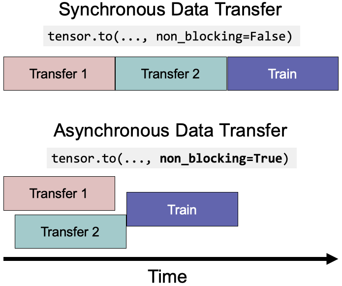
7. Use tensor.to(non_blocking=True) when it's applicable to overlap data transfers and kernel execution

Essentially, non_blocking=True allows asynchronous data transfers to reduce the execution time.
for features, target in loader:
    # these two calls are nonblocking and overlapping
    features = features.to('cuda:0', non_blocking=True)
    target = target.to('cuda:0', non_blocking=True)
    # This is a synchronization point
    # It will wait for previous two lines
    output = model(features)
#GPU #SaveTime
8. Fuse the pointwise (elementwise) operations into a single kernel by PyTorch JIT
Pointwise operations (see example list) include common math operations and usually are memory-bound. PyTorch JIT would automatically fuse the adjacent pointwise operations into one single kernel to save multiple memory reads/writes. (Pretty amazing, isn't it?) For example, the gelu function can be accelerated 4 times for a vector of one million by fusing 5 kernels into 1 (ref). More examples of PyTorch JIT optimization can be found here and here.
@torch.jit.script # JIT decorator
def fused_gelu(x):
    return x * 0.5 * (1.0 + torch.erf(x / 1.41421))
#CPU #GPU #SaveTime
9 & 10. Set the sizes of all different architectural designs and batch sizes as the multiples of 8
To maximize the computation efficiency of GPU, it's the best to ensure different architecture designs (including the input and output size/dimension/channel numbers of neural networks and batch size) are the multiples of 8 or even larger powers of two (e.g., 64, 128 and up to 256). It's because the Tensor Cores of Nvidia GPUs achieve the best performance for matrix multiplication when the matrix dimensions align to the multiples of powers of two. The matrix multiplication is the most-used operation and possibly the bottleneck, so it's the best we can make sure the tensors/matrices/vectors have the dimensions that are divisible by powers of two (e.g., 8, 64, 128, and up to 256).
These experiments have shown setting the output dimension and the batch size as the multiples of 8 (i.e., 33712, 4088, 4096) can accelerate the computation by 1.3x to 4x compared to the output dimension of 33708 and the batch sizes of 4084 and 4095, which are indivisible by 8. The acceleration magnitude depends on the process types (e.g., forward passes or the gradient calculations) and the cuBLAS versions. Especially, if you work on NLP, remember to check your output dimension, which is usually the vocabulary size.
Using the multiples of larger than 256 does not add more benefits but also does no harm. The settings depend on the cuBLAS and cuDNN versions and the GPU architecture. You can find the specific Tensor Core requirements of the matrix dimensions here. Since currently PyTorch AMP mostly uses FP16 and FP16 requires the multiples of 8, the multiples of 8 are usually recommended. If you have a more advanced GPU like A100, then you may choose the multiples of 64. If you are using AMD GPU, you may need to check AMD's documentation.
Besides setting batch size as the multiple of 8, we also maximize the batch size until it hits the memory limit of GPU. In this way, we can spend less time finishing an epoch.
#GPU #SaveTime
11. Use mixed precision for forward pass but not backward pass
Some of the operations do not need the precision of float64 or float32. Therefore, setting the operations for lower precision can save both memory and execution time. For various applications, Nvidia reported using mixed precision with the GPU with Tensor Cores can speed up by 3.5x to 25x (ref).
It is worth noting that usually the larger the matrix is, the more acceleration mixed precision achieves (ref1, ref2). In larger neural networks (e.g., BERT), one experiment has shown that the mixed precision can accelerate training by 2.75x and reduce 37% of memory usage (ref). The newer GPU devices with Volta, Turing, Ampere, or Hopper architectures (e.g., T4, V100, RTX 2060, 2070, 2080, 2080 Ti, A100, RTX 3090, RTX 3080, and RTX 3070) can benefit more from mixed precision because they have the Tensor Core architecture, which has special optimization and outperforms CUDA cores (ref).

To be noted, H100 with Hopper architecture, expected to release in the third quarter of 2022, supports FP8 (float8). PyTorch AMP may be expected to support FP8, too (current v1.11.0 has not supported FP8 yet).
In practice, you'll need to find a sweet spot between the model accuracy performance and speed performance. I did find mixed precision may reduce the model performance before, which depends on the algorithm, the data and the problem.
It's quite easy to leverage mixed precision in PyTorch with the automatic mixed precision (AMP) package. The default float point type in PyTorch is float32 (ref). AMP would save memory and time by using float16 for a group of operations (e.g., matmul, linear, conv2d, etc, see full list). AMP would autocast to float32 for some operations (e.g., mse_loss, softmax, etc, see full list). Some operations (e.g., add, see full list) would operate on the widest input type. For example, if one variable is float32 and another one is float16, the addition result would be float32.
autocast automatically applies precisions to different operations. Because loss(es) and gradients are calculated at float16 precision, the gradients might "underflow" and become zeroes when they are too small. GradScaler prevents underflow by multiplying the loss(es) by a scale factor, calculating the gradients based on the scaled loss(es), and then unscaling the gradients before the optimizer updates the weights. If the scaling factor is too large or too small and results in infs or NaNs, then the scaler would update the scaling factor for the next iteration.
scaler = GradScaler()
for features, target in data:
    # Forward pass with mixed precision
    with torch.cuda.amp.autocast(): # autocast as a context manager
        output = model(features)
        loss = criterion(output, target)
    # Backward pass without mixed precision
    # It's not recommended to use mixed precision for backward pass
    # Because we need more precise loss
    scaler.scale(loss).backward()
    # scaler.step() first unscales the gradients .
    # If these gradients contain infs or NaNs,
    # optimizer.step() is skipped.
    scaler.step(optimizer)
    # If optimizer.step() was skipped,
    # scaling factor is reduced by the backoff_factor in GradScaler()
    scaler.update()
You can also use autocast as a decorator for forward pass functions.
class AutocastModel(nn.Module):
    ...
    @autocast() # autocast as a decorator
    def forward(self, input):
        x = self.model(input)
        return x
#CPU #GPU #SaveTime #SaveMemory
12. Set gradients to None before the optimizer updates the weights
Setting gradients to zeroes by model.zero_grad() or optimizer.zero_grad() would execute memset for all parameters and update gradients with reading and writing operations. However, setting the gradients as None would not execute memset and would update gradients with only writing operations. Therefore, setting gradients as None is faster.
# Reset gradients before each step of optimizer
for param in model.parameters():
    param.grad = None
# or (PyTorch >= 1.7)
model.zero_grad(set_to_none=True)
# or (PyTorch >= 1.7)
optimizer.zero_grad(set_to_none=True)
#CPU #GPU #SaveTime
13. Gradient accumulation: update weights for every other x batch to mimic the larger batch size
This tip is about accumulating gradients from more data samples so that the estimation of gradients is more accurate and weights are updated more towards the local/global minimum. This is more helpful especially when the batch size is small (due to either a small GPU memory limit or a large data size per sample).
for i, (features, target) in enumerate(dataloader):
    # Forward pass
    output = model(features)
    loss = criterion(output, target)
    # Backward pass
    loss.backward()
    # Only update weights every other 2 iterations
    # Effective batch size is doubled
    if (i+1) % 2 == 0 or (i+1) == len(dataloader):
        # Update weights
        optimizer.step()
        # Reset the gradients to None
        optimizer.zero_grad(set_to_none=True)
#CPU #GPU #SaveTime
14. Turn off gradient calculation for inference/validation
Essentially, gradient calculation is not necessary for the inference and validation steps if you only calculate the outputs of the model. PyTorch uses an intermediate memory buffer for operations involved in variables of requires_grad=True. Therefore, we can avoid using additional resources by disabling gradient calculation for inference/validation if we know we don't need any gradient-involved operations.
# torch.no_grad() as a context manager:
    with torch.no_grad():
    output = model(input)
# torch.no_grad() as a function decorator:
@torch.no_grad()
def validation(model, input):
    output = model(input)
return output
#CPU #GPU #SaveTime #SaveMemory
15. torch.backends.cudnn.benchmark = True
Setting torch.backends.cudnn.benchmark = True before the training loop can accelerate the computation. Because the performance of cuDNN algorithms to compute the convolution of different kernel sizes varies, the auto-tuner can run a benchmark to find the best algorithm (current algorithms are these, these, and these). It's recommended to use turn on the setting when your input size doesn't change often. If the input size changes often, the auto-tuner needs to benchmark too frequently, which might hurt the performance. It can speed up by 1.27x to 1.70x for forward and backward propagation (ref).
torch.backends.cudnn.benchmark = True#GPU #CNN #SaveTime
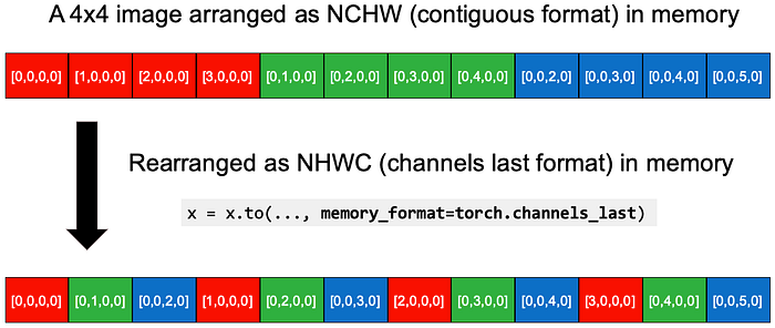
16. Use channels_last memory format for 4D NCHW Tensors

Using the channels_last memory format saves images in a pixel-per-pixel manner as the densest format in memory. Original 4D NCHW Tensors are clustered by each channel (Red/Greed/Blue) in memory. After the conversion, x = x.to(memory_format=torch.channels_last), the data is reorganized as NHWC (channels_last format) in memory. You can see each pixel of the RGB layers is closer. This NHWC format has been reported to gain 8% to 35% speedup with AMP of FP16 (ref).
Currently, it is still in beta, and only supports 4D NCHW Tensors and a group of models (e.g., alexnet, mnasnet family, mobilenet_v2, resnet family, shufflenet_v2, squeezenet1, vgg family, see full list). But I can definitely see this would become a standard optimization.
N, C, H, W = 10, 3, 32, 32
x = torch.rand(N, C, H, W)
# Stride is the gap between one element to the next one
# in a dimension.
print(x.stride()) # (3072, 1024, 32, 1)
# Convert the tensor to NHWC in memory
x2 = x.to(memory_format=torch.channels_last)
print(x2.shape)  # (10, 3, 32, 32) as dimensions order preserved
print(x2.stride())  # (3072, 1, 96, 3), which are smaller
print((x==x2).all()) # True because the values were not changed
#GPU #CNN #SaveTime
17. Turn off bias for convolutional layers that are right before batch normalization
This works because mathematically the bias effect would be canceled out by mean subtraction of the batch normalization. We can save the model parameters, run time, and memory.
nn.Conv2d(..., bias=False)#CPU #GPU #CNN #SaveTime #SaveMemory
18. Use DistributedDataParallel instead of DataParallel
It's always prefer DistributedDataParallel over DataParallel for multi-GPU even with only a single node because DistributedDataParallel applies multiprocessing and creates a process for each GPU to bypass Python Global Interpreter Lock (GIL) and speed up.
#GPU #DistributedOptimizations #SaveTime
Summary
In this post, I made a checklist and provided code snippets for 18 PyTorch tips. Then I explained how and why they work one by one in various aspects including data loading, data operations, model architecture, training, inference, CNN-specific optimizations, and distributed computing. Once you deeply understand how they work, you may be able to find the common principles that are applicable to deep learning modeling in any deep learning framework.
Hope you enjoy the more efficient PyTorch and learn something new!
Please leave comments and other tips below if you have any. Thank you.
I am Jack Lin, a senior data scientist at C3.ai, and I'm passionate about deep learning and machine learning. You can check out my other articles on Medium!

