When it comes to applying machine learning to physical system modeling, it is more and more common to see practitioners moving away from a pure data-driven strategy, and starting to embrace a hybrid mindset, where rich prior physical knowledge (e.g., governing differential equations) is used together with the data to augment the model training.

Under this background, physics-informed neural networks (PINNs) have emerged as a versatile concept and led to many success stories in effectively solving real-world challenges.

As a practitioner who is eager to adopt PINNs, I am keen on learning both the latest developments in training algorithms, as well as the novel use cases of PINNs for real-world applications. However, a pain point I often see is that, although there are abundant research papers/blogs summarizing effective PINN algorithms, overviews of novel use cases of PINNs can rarely be found. One obvious reason is that, unlike the training algorithms which are domain-agnostic, reports of PINN use cases are scattered in various engineering domains and not readily accessible for a practitioner who is usually an expert in one specific domain. As a consequence, I often found myself reinventing the wheel as my ways of using PINNs have already been well addressed by practitioners in another field.

It is exactly my journey and experiences that have sparked the idea of writing this blog: here, I strive to break the information barrier across different engineering domains and distill the recurring functional usage patterns of PINNs. I hope that this review will inform practitioners from different domains about what's possible with PINNs and inspire new ideas for interdisciplinary innovation.

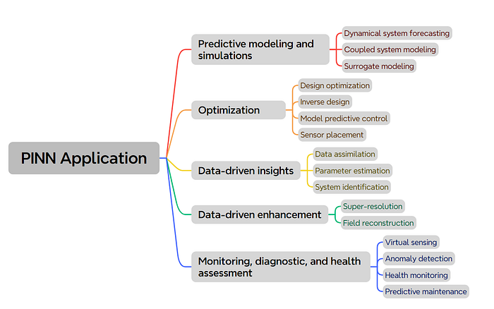
Toward that end, I have extensively reviewed PINN research papers in the past three years and came up with the following 5 main usage categories:

• Predictive modeling and simulations
• Optimization
• Data-driven insights
• Data-driven enhancement
• Monitoring, diagnostic, and health assessment

In the following, we will introduce in turn the common PINN usages under each of these categories. For each category, we will discuss the problem statement, why PINNs are useful, and how PINNs can be implemented to address the problem. For each type of problem, we will ground our discussion with a concrete use case published in the literature.

A roadmap of this blog post is shown below:

Disclaimer: The categorization of PINN usage patterns dicussed in this blog only represents my current, limited experience with PINNs. By no means it provides a complete picture. Nevertheless, it could serve as a good starting point for appreciating the wide applications of PINNs.

This blog solely focuses on the applications of PINNs. If you are also interested in learning the algorithmic side of PINNs, feel free to check out my blog series here: Unraveling the Design Pattern of Physics-Informed Neural Networks.

With that in mind, let's get started!

Table of Content · 1. Predictive modeling and simulations ∘ 1.1 PINN Fundamentals ∘ 1.2 Dynamical system forecasting ∘ 1.3 Coupled system modeling ∘ 1.4 Surrogate modeling ∘ 1.5 Summary · 2. Optimization ∘ 2.1 Design optimization ∘ 2.2 Inverse design ∘ 2.3 Model predictive control ∘ 2.4 Sensor placement ∘ 2.5 Summary · 3. Data-Driven Insights ∘ 3.1 PINN for inverse problem ∘ 3.2 Parameter estimation ∘ 3.3 System identification ∘ 3.4 Data assimilation ∘ 3.5 Summary · 4. Data-Driven Enhancement ∘ 4.1 Field reconstruction ∘ 4.2 Super-resolution ∘ 4.3 Summary · 5. Monitoring, Diagnostic, Health Assessment ∘ 5.1 Virtual sensing ∘ 5.2 Anomaly detection ∘ 5.3 Health monitoring ∘ 5.4 Predictive maintenance ∘ 5.5 Summary · 6. Conclusion

1. Predictive modeling and simulations

In computational science and engineering, predictive modeling and simulations are the most fundamental tasks and this is also where PINNs were widely employed. In this section, we will first briefly review the basic theory of PINNs to set the stage, followed by discussing three prominent application subcategories, i.e., dynamical system forecasting, coupled system modeling, as well as surrogate modeling.

1.1 PINN Fundamentals

For predictive modeling and simulations, our ultimate goal is to obtain the values of physical quantities (e.g., velocity u, pressure p, temperature T, etc.) at any temporal/spatial coordinates (i.e., t, x, y) within the considered domain.

If we adopt a neural network approach to predict those quantity values, our neural network would take as inputs the temporal/spatial coordinates (i.e., t, x, y), and output the quantities of interests (e.g., u, p, T, etc.).

But how do we train this neural network?

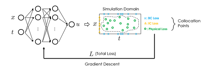
Physics-informed neural networks introduced a delightfully simple idea: the residuals of the governing differential equations, which are calculated by supplying the predicted quantities into the governing equations, are used to construct the loss term for model training. By minimizing this loss term, we effectively make the trained network obey the underlying physics.

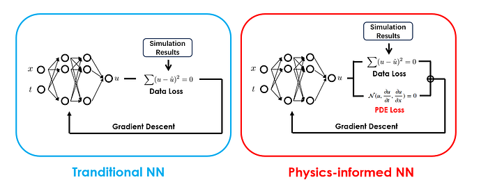
In practical implementations, those residuals are calculated at a set of randomly sampled temporal/spatial coordinates known as collocation points. By using automatic differentiation (which is readily available in nowadays deep learning frameworks), the derivatives of the outputs (i.e., physical quantities) at the selected collocation points can be easily computed.

PINNs possess the following characteristics:

• Compared to the traditional numerical simulation approaches, PINNs are mesh-free. This enables PINNs to easily handle complex simulation domains, reduce manual effort in simulations, and potentially improve computational efficiency.
• Thanks to the universal approximation capability, PINNs are well-suited for modeling complex and nonlinear systems where traditional methods may struggle.
• Compared to the traditional paradigm of supervised learning, PINNs are in principle data-free, i.e., their training does not require collecting input-output pairs, i.e., (t, x, y)-(u, p, T), but entirely based on fulfilling the governing differential equations. However, if scarce data is available, PINNs can also effectively assimilate that. We will come back to this point in later sections.

In the following, we will see how those characteristics enable effective predictive modeling and simulations.

1.2 Dynamical system forecasting

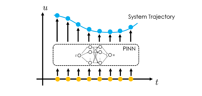
One common application of PINNs is for forecasting the state evolution of the dynamical systems.

Partial differential equations (PDEs) and ordinary differential equations (ODEs) are commonly used to mathematically describe how the physical system evolves over time. Meanwhile, we note that PINNs are essentially a PDE/ODE solver, as they predict the values of physical quantities at any spatial & temporal coordinates within the simulation domain. Therefore, by using PINNs to solve the PDE/ODE in question, we can obtain the full trajectory of state evolution of the dynamical systems, given some initial conditions.

📋 Case study

In Antonelo et al. [Physics-Informed Neural Nets for Control of Dynamical Systems], the authors investigated forecasting the state evolution of a Van der Pol oscillator (which is widely used in seismology and biology modeling) and a four tanks system (which is a popular benchmark for multivariate control system), with both dynamical systems governed by ODEs.

Standard PINN strategy can effectively achieve the forecasting goal: the neural network takes as an input time t and outputs the system state u. By minimizing the ODE residuals calculated at randomly sampled collocation points (t₁, t₂, …) within the modeling timespan [0, T], the neural network can be properly trained and provides accurate predictions of u given any input t within [0, T]. This way, we have obtained the desired state evolution trajectory.

To forecast system states u beyond the initial time interval [0, T], the authors proposed to include the initial condition u₀ as an extra input (together with t) of the PINN. This way, when we finish the prediction for [0, T], given some known initial condition u₀, we can use the predicted state u at t=T as the new initial condition u₀. Now with this updated initial condition fed to the neural network, when we vary t between [0, T], we are effectively predicting the system states in the next time interval [T, 2T].

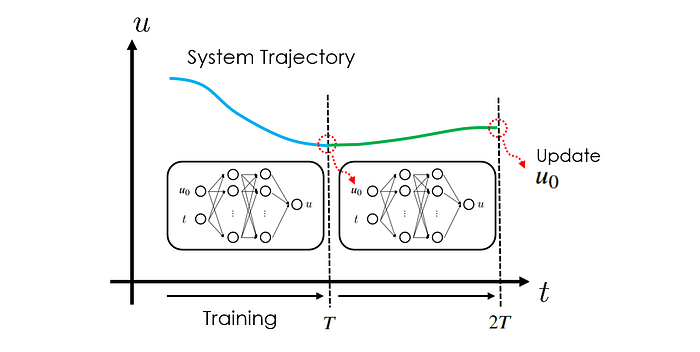
This iterative process allows the network to extend its forecasting horizon to longer time intervals. According to the authors' experiments, they observed that PINN's way of forecasting state evolution delivers faster results than the conventional numerical solvers.

Note that in the paper, the authors mainly developed this long-time forecasting capability for control purposes. We will come back to that in Section 2,3: Model Predictive Control.

1.3 Coupled system modeling

Another area where PINNs are especially useful is predictive modeling and simulations for coupled systems (e.g., multi-phase systems, multi-physics systems, etc). Such systems are characterized by multiple interacting components and/or phenomena, and they are commonly seen in various engineering fields.

Traditional modeling approaches may encounter difficulties in simulating coupled systems, as different components may require specific numerical treatments. In addition, the computational cost may be high due to the need to simultaneously solve multiple interconnected differential equations.

PINNs, on the other hand, are well-suited for such systems. Thanks to the high flexibility and expressivity of the neural network, various types of governing differential equations can all be learned under one unified framework. This allows the PINN approach to more easily capture the complex interactions presented in the coupled system.

📋 Case study

Cai et al. [Physics-Informed Neural Networks for Heat Transfer Problems] investigated a two-phase Stefan problem, which is a common type of problem in heat transfer and includes use cases of chemical vapor deposition, welding, semiconductor design, and more. This type of problem features dynamic interactions between different material phases, resulting in moving boundaries or free interfaces. As a result, this problem poses a great challenge to traditional numerical methods.

To adapt PINN to simulate the two-phase Stefan problem, i.e., obtaining the T₁(x, t) (temperature distribution within the first phase), T₂(x, t) (temperature distribution within the second phase), and s(t) (location of the moving interface between the two phases), the authors proposed a dual-network solution: one neural network takes in as input the spatial & temporal coordinates (x, t) and outputs T₁ and T₂, while the other neural network takes in as input the temporal coordinates t and outputs s.

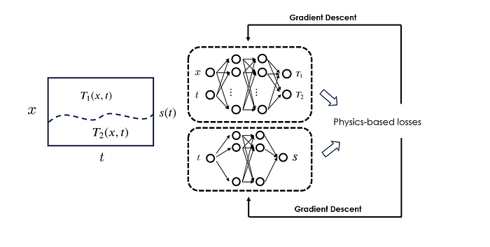
Those two networks are trained jointly under a shared physics-informed loss function. This loss function consists of 5 terms: heat transfer PDE residuals for phases 1 and 2, respectively, temperature continuity condition across the interface, energy balance across the interface, and initial location for the interface.

In the paper, the authors showed that their PINN strategy accurately predicted the temperature fields and the dynamic interface in the two-phase Stefan problem, therefore suggesting PINN's potential utility in modeling complex, coupled systems.

1.4 Surrogate modeling

For predictive modeling and simulations, we are usually not done with just getting the simulation results under one specific set of conditions. Instead, we would like to ask "what-if" questions to examine the system's response given different sets of, e.g., boundary conditions, initial conditions, material properties, etc.

To achieve this goal with traditional numerical methods, we would need to run simulations many times where each run corresponds to one specific setting (i.e., BC, IC, material properties, etc.) that the analyst would like to investigate. Overall, this leads to a very time-consuming process and hinders us from efficiently understanding the system's characteristics.

Enter surrogate modeling.

Surrogate modeling refers to the practice of building machine learning models to approximate the input-output relationship conveyed by the simulator. It starts with collecting a paired input-output dataset by running the simulations at carefully sampled input locations, followed by training the machine learning model on the collected dataset. Once this surrogate model is trained, it can predict the output for the given input with an accuracy close to the original simulator, but with only a fraction of the computational cost.

To learn more about surrogate modeling, feel free to check one of my most-viewed blogs here: An introduction to Surrogate modeling, Part I: fundamentals

Conventionally, the surrogate model and the simulator are considered two separate things, with the surrogate model attempting to emulate the simulator. The advent of PINNs turns this concept around. In fact, since PINNs are machine learning models trained by solving the governing differential equation, by design, PINNs function as both a surrogate model and a simulator.

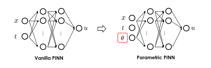
To make PINN a more useful surrogate model, a commonly used trick is to include system parameters we wish to examine as extra inputs alongside the spatial & temporal coordinates (x, t). This way, the network predictions of the system states u at (x, t) will now be conditioned on the given input of parameters of interest. As a result, answering "what-if" questions becomes straightforward as we only need to query the PINN with different parameter settings to obtain the variations of the system's response. This enhanced form of PINNs is commonly known as parametric PINNs.

📋 Case study

Würth et al. [Physics-informed neural networks for data-free surrogate modeling and engineering optimization — An example from composite manufacturing] developed parametric PINNs to simulate the thermochemical curing process of composite materials. Heat transfer equations and curing kinetics equations were used as the differential equations to describe the physical process.

Besides the conventional (x, y, t) inputs, physical parameters related to the process, e.g., processing temperatures in the boundary condition and thermal properties of the material are considered as extra inputs to feed into the neural network. This is the key step that makes a standard PINN parametric.

In the paper, the authors demonstrated that the trained parametric PINN can accurately predict the temperature distribution and degree of curing within the composite material under a wide range of processing conditions, thus greatly enhancing process understanding and effectively supporting process optimization.

1.5 Summary

In this section, we introduced the use of PINNs for predictive modeling and simulation, which forms one of the fundamental tasks in computational science and engineering. We covered three key areas: dynamical system forecasting, coupled system modeling, as well as surrogate modeling. We showed that PINNs excel in these domains by offering enhanced forecasting accuracy for dynamical systems, efficient modeling of complex interactions in coupled systems, and rapid "what-if" analysis through surrogate modeling.

Now, let's move on to the next category: optimization.

2. Optimization

In this section, we take a look at how PINNs can be instrumental in optimization, which is another important task category in computational science and engineering. Specifically, we will review four application patterns in this category: design optimization, inverse design, model predictive control, and sensor placement.

2.1 Design optimization

For system process design, the goal of design optimization is to find the best system process parameters that deliver the best efficiency and performance while meeting specific constraints.

In practice, design optimization is conducted in an iterative manner, where optimization algorithms (e.g., L-BFGS, Genetic algorithm, etc.) update the design parameters towards better objective values at each iteration step. Usually, calculating objective values calls for running computationally expensive physical simulations. Unfortunately, for complex systems, many optimization iterations may be required until the objective is optimized, thus leading to a very time-consuming process.

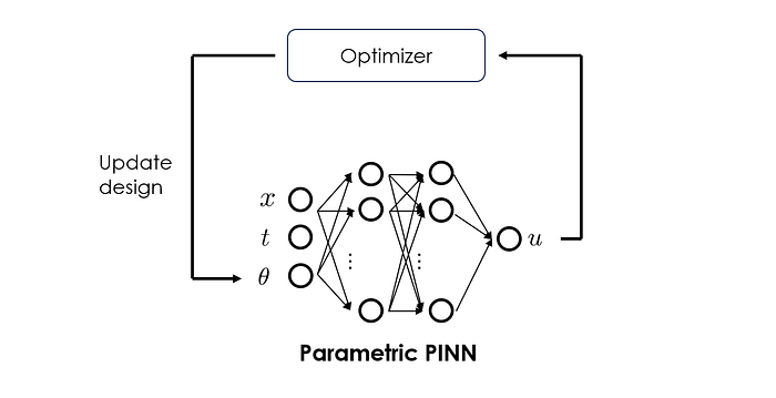
To combat the low-efficiency issue in design optimization, a popular approach adopted by practitioners is surrogate modeling. More specifically, we can first train a machine-learning-based surrogate model to approximate the slow physical simulations. Then, we integrate this trained surrogate model into the optimization loop such that the surrogate model, instead of the original simulator, will be called when evaluating the objective function. This way, each optimization iteration can be completed in a much shorter time, therefore greatly accelerating the overall optimization process.

Earlier, we mentioned that PINNs can be upgraded to be parametric, thus paving the way for acting as a surrogate model. This is exactly how PINNs could be leveraged for efficient design optimization.

📋 Case study

Cai et al. [Physics-Informed Neural Networks for Heat Transfer Problems] explored optimizing a heat sink design on a Nvidia GPU chip using parametric PINN. Here, the optimization objective is to minimize the peak temperature of the chip while satisfying a maximum pressure drop constraint. To use PINNs to accelerate the design optimization, parameters associated with the fin geometry of the heat sink are taken as the extra inputs to the PINN. This allows PINNs to quickly explore the design space, therefore improving the efficiency of the overall optimization.

The authors showed that PINNs can solve the problem faster than traditional solvers by several orders of magnitude.

2.2 Inverse design

In the field of computational science and engineering, inverse design refers to the scenario where the desired system performance is specified first, and then the system configurations that achieve this outcome are determined. Technically, it usually involves applying optimization algorithms to search for the optimal design parameters that meet pre-defined targets.

Addressing inverse design problems relies heavily on simulations of how different designs will perform. However, as exploring a very large design space is usually required, traditional numerical ODE/PDE simulators that are slow to run may be inadequate to efficiently identify the optimal design.

PINNs, on the other hand, are well-suited for solving the inverse design problem. There are a couple of reasons:

• PINNs can significantly speed up simulations compared to traditional numerical methods.
• PINNs are capable of efficiently handling high-dimensional problems and nonlinear dynamics, which is often the case in inverse design scenarios.
• PINNs are fully differentiable, meaning that we can easily compute the gradients of some objective with respect to the input parameters (e.g., using FensorFlow's tf.GradientTape). This opens the door for gradient-based optimization algorithms, which may facilitate more efficient searching in the design space.

📋 Case study

Lu et al. [Physics-Informed Neural Networks with Hard Constraints for Inverse Design] investigated using PINNs to perform topology optimization for a holography problem in optics.

In this problem, the goal is to design the permittivity map ε(x, y) of a scattering slab, such that it can scatter light in a way that the transmitted wave pattern forms a targeted shape f(x, y). This is a typical form of inverse design problem.

To solve this problem, the authors constructed three neural networks, where the first two take (x, y) as inputs and output the real and imaginary parts of the electromagnetic wave, respectively, and the final one takes (x, y) as inputs and outputs the permittivity map ε(x, y) (i.e., our design variables). Those three networks are trained jointly with a common loss function.

What makes the paper unique is the way how the loss function is constructed. As proposed by the authors, the loss function consists of two terms:

• The first term is the usual PDE residual loss, which is calculated by substituting the three outputs predicted by the three networks into the Maxwell function.
• The second term is target mismatch, which is calculated by comparing the predicted transmitted wave pattern (as a function of the three network outputs) to the target pattern f(x, y).

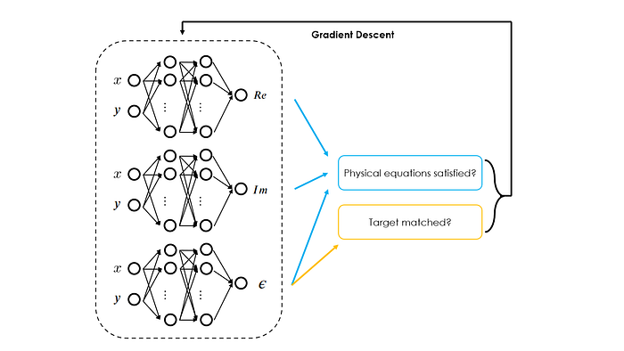
By minimizing those two losses simultaneously, the authors showed that it is possible to obtain a target design while still adhering to the constraints of Maxwell's equations. The authors further demonstrated that compared to the conventional inverse design approaches, the PINN-based approach is easier to implement and the design found by PINNs is simpler and smoother, therefore showing the effectiveness of PINNs in addressing this type of problem.

2.3 Model predictive control

Our ultimate goal in predicting and understanding the system dynamics is to control the system such that it behaves as we desire. For that, we need control algorithms.

Over the years, many control algorithms have been proposed by practitioners. More recently, model predictive control (MPC) has emerged as a promising control technique that enjoys growing popularity in various industries. At its core, MPC uses a model of the target dynamical system and it operates in the following steps:

• it predicts the future behavior of the system over a finite horizon.
• it optimizes the actuator's control signals based on this prediction to minimize some loss function (e.g., minimize the discrepancy between the predicted state trajectory and the reference state trajectory), while observing the constraints, e.g., limits on actuators.
• it repeats the above two steps for the next time horizon.

In practice, however, solving this optimal control problem iteratively can be quite computationally intensive, as the underlying optimization problem involves evaluating a possibly expensive simulation model that describes the system dynamics. As a result, how to improve the optimization efficiency such that the real-time optimal control signal can be derived becomes the key question to address in realistic MPC implementations.

It didn't take practitioners long to realize that PINNs can be quite useful for realizing MPC. Similar to what we have discussed in Section 2.1 Design optimization, PINNs can be upgraded to a parametric one and effectively serve as surrogate models. By doing so, they can significantly reduce the computational cost when evaluating system dynamics under different control settings, thus better facilitating the optimization algorithms to explore the parameter space and locate the optimal solution.

📋 Case study

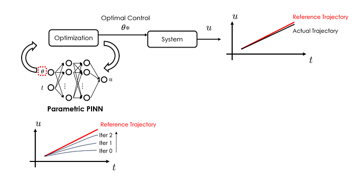
Sanyal et al. [RAMP-Net: A Robust Adaptive MPC for Quadrotors via Physics-informed Neural Network] developed a PINN-based MPC strategy for high-speed drone navigation.

In their work, the authors used PINN to efficiently solve the governing ordinary differential equation (ODE) that describes the drone's flight dynamics. To enable control optimization, in addition to the time t, the PINN also took as inputs the control variables (i.e., quadrotor thrusts) and the initial state values. The developed PINN was later plugged into the MPC formulation to identify the optimal values of the control variables that can generate the flight trajectory that is as close as possible to the reference one.

What's also interesting to mention is that in their work, both governing ODE and observational data were used to train the PINN. The motivation for doing that is that the governing ODE, due to physical simplifications, cannot fully capture the system dynamics. The extra data loss term could help PINN to overcome the induced model uncertainty, therefore being more adaptive to realistic situations.

2.4 Sensor placement

When performing physical experiments to investigate the system characteristics, the placement of sensors is usually one of the crucial decisions to make. Depending on how many and where sensors are deployed, the obtained data quality and relevancy, as well as the induced financial cost would be drastically different. To minimize the cost, it is common in practice to first perform some numerical simulations to inform the sensor placement strategy.

PINNs can be quite useful in this context: not only because they can deliver efficient simulation compared to the traditional numerical methods, but also because they open the door for algorithmically determining the optimal sensor placement strategy.

📋 Case study

Cai et al. [Physics-Informed Neural Networks for Heat Transfer Problems] investigated the sensor placement issue given a forced heat convection scenario, which is commonly encountered in various industrial systems (e.g., cooling systems for electronics, HVAC systems, etc). The goal here is to determine the most informative locations to deploy sensors so that the temperature distributions can be accurately reconstructed.

What's novel about this work is that the authors proposed a simple yet effective strategy for selecting the best sensor locations: they first use a standard PINN to simulate the flow field. Afterward, they simply calculate the residuals of the governing incompressible Navier-Stokes equations for temperature, and the location corresponding to the maximum residual value is then selected as the place to deploy the sensor.

This approach makes sense as the temperature PDE residual reflects how well the current temperature prediction fulfills the governing PDE. When reaching a maximum PDE residual, it indicates that the PINN struggles the most in making accurate predictions at this position. Therefore, by placing one sensor here, we can extract the most value from the measurement data to refine and improve the PINN's predictive accuracy.

In practice, the above-mentioned strategy is implemented in an iterative manner, such that the sensors are added sequentially. The authors showed that the accuracy of the PINN's temperature prediction improved significantly even with one round of active sensor placement iteration.

Note that the main purpose of this work is to use PINNs to reconstruct the flow field based on sparse measurements. We will come back to this type of problem later in section 4.

2.5 Summary

In this section, we introduced the use of PINNs for optimization, which forms another important task in computational science and engineering. We covered the following three key areas:

• Design optimization: Parametric PINNs can serve as an accurate and efficient surrogate model to accelerate the optimization process.
• Inverse design: PINNs facilitate highly efficient topology optimization for complex systems and ensure that the design property matches the pre-defined target and the design is indeed a physically plausible one.
• Sensor placement: PINN's "weakness" can be turned into a strength, in the sense that the positions where PINN struggles to fulfill the governing equation are promising locations for sensor placement.

Now, let's move on to the next category: data-driven insights.

3. Data-Driven Insights

For many real-world complex systems, we rarely have complete knowledge about them: sometimes, we may not know the form of the underlying governing PDEs; other times, we would be lucky enough to know the exact PDE forms. However, some parameters (e.g., material properties) in the PDE may still be hidden from us.

Fortunately, we can observe the system and collect the corresponding measurement data. As a result, the main theme of data-driven insights is to use algorithms to extract insights about the system dynamics based on the observed system data.

PINNs perfectly fit this theme as PINNs are both a physics-informed and data-driven method. So, in this section, let's take a look at how PINNs can be used for deriving insights from the data with parameter estimation, system identification, and data assimilation.

From a technical perspective, we are now entering the world of inverse problems. Therefore, before we discuss any specific PINN use cases, it would be a good idea to first briefly review PINN's strategy for performing inverse analysis.

3.1 PINN for inverse problem

When considering forward problems, we typically look at how information propagates from causes to effects. Inverse problems, on the other hand, work oppositely by reversing the flow of information from effects to causes. These problems often arise in situations where the underlying system is unknown or only partially known, and our goal is to infer those unknowns from the observational data.

Traditionally, inverse problems are typically approached as optimization challenges. Take parameter estimation as an example (e.g., estimating system property parameters in the governing PDE): in the conventional optimization framework, at each iteration step, the optimizer would "tweak" those unknown parameters such that, when we substitute those adjusted parameters into the PDE and simulate the PDE, we would obtain results that align closer with the observational data. In this process, however, PDE simulation and parameter optimization are treated as two separate operations.

PINNs introduced a significant paradigm shift by merging these two operations: since solving PDE equates to optimizing the weights & biases of a neural network in the context of PINN, we might as well just optimize the network parameters (i.e., weights & biases) and the unknown system parameters simultaneously, such that the predicted outcomes can be both data-consistent and physically plausible. This is the core idea of using PINNs for solving inverse problems.

3.2 Parameter estimation

Earlier we mentioned that for estimating parameters with PINNs, we could optimize the system parameters alongside the network's weights and biases. In terms of implementation, we need to:

• include system parameters to be estimated as trainable parameters. By doing so, the gradients of the loss with respect to those system parameters will be backpropagated to update the parameters. Technically, this can be done by creating a dummy neural network layer that holds those parameters but does nothing besides passing inputs to outputs without any modification.
• expand the loss function such that it contains both the standard PDE loss and an extra data loss term. This data loss term is a standard supervised loss, such as the mean squared error between the network predictions and the observations.

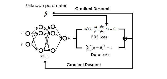
Generally, both PDE loss and data loss are functions of the parameters we desire to estimate. Therefore, by jointly optimizing these loss terms, we guide the network to find the parameter values that not only satisfy the governing PDEs but also align closely with the observational data.

📋 Case study

Grimm et al. [Estimating the Time-dependent Contact Rate of SIR and SEIR Models in Mathematical Epidemiology Using Physics-Informed Neural Networks] leveraged PINNs for parameter estimation within the context of epidemiology. Specifically, the authors estimated the contact rate (which is a key parameter in the virus-spreading ODE) from the observed COVID-19 pandemic data.

By jointly optimizing the PINN network parameters and the contact rate parameter, the authors showed the feasibility of accurately and efficiently estimating the contact rate.

What's novel about this work is that the authors implement their algorithms in an online manner: essentially, they perform the parameter estimation only over a short time interval, within which the contact rate is assumed to be constant. And they can quickly update the estimation when new data becomes available. This online approach to parameter estimation is particularly valuable, as it enables a better understanding of how the contact rate changes over time, which is a crucial factor that informs public health policies.

3.3 System identification

Besides unknown parameters, we may also have unknown terms in the governing ODE/PDEs for complex systems. For example, in the following ODE that models animal population growth p under limited resources, we may only know the precise functional form of the H(·) term (as it is controlled by human activity), but do not know the exact functional form of the natural dynamics term f(·), which describes the population growth without human intervention.

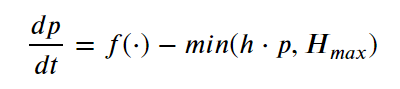
This process of recovering the unknown ODE/PDE terms from the observational data is what we call system identification.

In the framework of PINNs, solving system identification problems shares the same core idea as addressing the parameter estimation problems we discussed earlier. Essentially, we can approximate those unknown terms with an auxiliary neural network (that is to say, we surrogate the input-output relationship of the unknown terms with a neural network), and train this neural network with the main PINN network together to minimize the physical PDE loss and data loss.

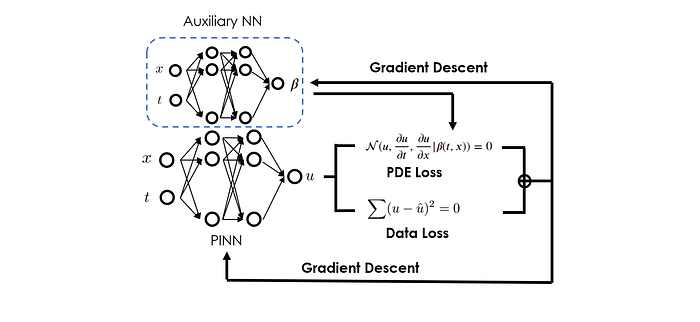
Similar to the parameter estimation case, in practice, we could also implement a custom layer to hold this auxiliary neural network in the overall PINN model. However, unlike in parameter estimation where the custom layer does no operation besides holding the parameters to be estimated, here, the custom layer would call the auxiliary neural network to propagate information from input to output. As a result, the final loss will also depend on the weights & biases of the auxiliary neural network, which gives us the mechanism to optimize them.

For a tutorial on using PINNs for solving system identification problems, feel free to check out my blog here: Discovering Differential Equations with Physics-Informed Neural Networks and Symbolic Regression.

📋 Case study

Zhang et al. [Discovering a reaction-diffusion model for Alzheimer's disease by combining PINNs with symbolic regression] looked into modeling the spatiotemporal concentration of misfolded tau protein, which plays a crucial role in the progression and pathology of Alzheimer's disease.

The challenge encountered in the study is that, although it is known that a reaction-diffusion type of PDE governs the distribution of misfolded tau protein, the specific reaction term in the equation is not known.

To tackle this challenge, the authors configured two neural network models, with one being the main PINN model and the other one being the auxiliary model that "surrogates" the effect of the unknown reaction term. By training both models concurrently using both the physics-informed loss (i.e., the PDE loss) and the clinical data, the authors accurately identified the unknown reaction term that is both data-consistent and physically plausible.

What's also interesting about the work is that the authors further leveraged a technique called symbolic regression to distill an analytical expression from the trained auxiliary network model. This way, the concentration pattern of misfolded tau protein can be transparently explained, thus informing early diagnosis and treatment plans.

3.4 Data assimilation

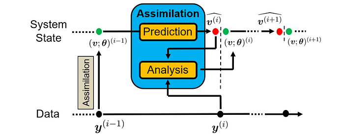
Data assimilation refers to the practice of combining observational data with an ODE/PDE model to better estimate the parameters and states of a physical system, which will later be used for making accurate forecasts for system dynamics. Data assimilation is commonly implemented in an online manner, where model predictions are updated as new observational data becomes available.

Similar to the parameter estimation and system identification tasks, data assimilation also solves an inverse problem. However, data assimilation emphasizes more on estimating the states of the system from the available model and data.

📋 Case study

He et al. [Physics-Informed Neural Networks for Multiphysics Data Assimilation with Application to Subsurface Transport] investigated a data assimilation problem in transport modeling in heterogeneous porous media, which finds wide applications in environmental engineering. Specifically, the authors employed PINNs to assimilate sparse measurement data to estimate the states of hydraulic conductivity, hydraulic head, as well as concentration.

The authors constructed three separate neural networks corresponding to each of the three estimation targets. Those networks are trained jointly by minimizing both a PDE loss term, which is computed by substituting the three estimated targets (and their derivatives) to the Darcy flow equation and the advection-dispersion equation, as well as a standard supervised data loss term to align the estimated targets with the associated measurements.

The authors showed that the PINN approach delivered an accurate estimation of the target states, and provided an attractive alternative to pure data-driven approaches when the measurement data is sparse.

3.5 Summary

In this section, we explored the use of PINNs for addressing inverse problems, i.e., deriving insights about the underlying system from associated measurement data. Under this theme, we discussed three specific tasks that are commonly seen in various computational engineering domains: parameter estimation, system identification, and data assimilation. Being both a data-driven and a physics-informed approach, we have seen that PINNs are perfectly capable of solving those tasks and ensuring the estimations are not only data-consistent but also physically plausible.

Now, let's move on to the next category: data-driven enhancement.

4. Data-Driven Enhancement

Having explored adopting a data-driven mindset to derive new physical insights, we now move to a related, yet slightly different task usually seen in computational science and engineering: data-driven enhancement.

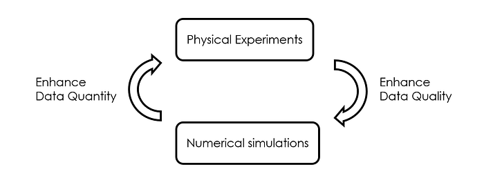
Often, the cost of conducting physical experiments and acquiring field measurement data is exceedingly high. Meanwhile, computer simulations are known to be incapable of fully reproducing reality, due to inevitable simplifications made along the way. As a result, it is natural to seek methods that can synergize the measurement data and simulation data to achieve the optimal trade-off between the cost of data generation and data quality, thus facilitating better handling of downstream tasks, such as real-time decision-making.

Therefore, we can view the enhancement from both perspectives: from the physical experiment's point of view, we can use simulation to complement the experiments, thus enhancing the data quantity; from the numerical simulation's point of view, we can leverage measurements to complement the simulation, thus enhancing the data accuracy.

PINNs, given their unique feature of being both a physics-informed approach and a data-driven approach, nicely fit with this theme and can deliver our goal of data-driven enhancement. So, in this section, we delve into two important applications within this category, i.e., field reconstruction and super-resolution, where PINNs play a pivotal role.

4.1 Field reconstruction

For the task of field reconstruction, we aim to enhance the simulation of a physical field by incorporating sparse or incomplete field measurements. In this setting, the collected measurement data can be used to effectively "correct" the numerical simulation, thus enhancing the accuracy of the simulation.

The way that PINNs can help achieve this goal is by a simple addition of the data loss term (alongside the standard PDE loss), which quantifies the deviation between the PINN's predictions and the observed ground truth. Thanks to this extra loss term, we directly provide supervision signals to the PINN training, which not only facilitates a faster convergence but also allows PINNs to accurately reconstruct the physical field.

📋 Case study

Rui et al. [Reconstruction of 3D flow field around a building model in wind tunnel] applied PINNs to solving building wind engineering problems and investigated reconstructing the flow field around the scale model of a building in a wind tunnel.

The authors incorporated only the measured near-wall velocity data into the PINN's training to mimic realistic applications. They compared the reconstructed field to other measurements not used for the training, and showed that with only a small amount of measured data, the missing airflow information within the whole computational domain can be well recovered.

4.2 Super-resolution

Super-resolution (SR) represents another interesting type of task in the category of data-driven enhancement. As its name implies, this task aims to enhance the data resolution by extracting finer-scale information from existing low-resolution data. There are usually strong motivations for doing SR: in practice, field observations (e.g., satellite images) are often limited to coarse spatial and temporal grid resolution and thus may fail to support downstream analysis and decision-making.

In the context of PINNs, super-resolution can also be achieved via constructing a hybrid loss function, i.e., a data loss term to ensure the model predictions match with the available low-resolution data, and a standard PDE loss term, to enforce the physical consistency. After training, PINNs can be used to generate field predictions at a much finer resolution, thus surpassing the limitations of the original data collection methods.

📋 Case study

Wang et al. [Physics-Informed Neural Network Super Resolution for Advection-Diffusion Models] investigated the problem of reconstructing high-resolution images from lower-resolution satellite imagery of atmospheric pollution plumes.

In this work, the authors configured a CNN model with residual dense blocks that takes as input a low-resolution image and outputs the corresponding high-resolution one. The training was conducted under a hybrid loss function, which consists of a pixel loss term and a PDE loss term (residuals of an advection-diffusion equation for plume simulation).

The authors showed that compared to the traditional interpolation-based SR techniques, the PINN-based strategy significantly increased the reconstruction accuracy. In addition, the authors also demonstrated that PINN-based super-resolution is robust against missing pixels (e.g., cloud cover, etc) and works well even when a large portion of pixels is missing.

4.3 Summary

In this section, we looked at the use of PINNs for achieving data-driven enhancement. We viewed the enhancement from two perspectives:

• Leveraging the sparse measurements to enhance the accuracy of the simulation. In this direction, we discussed the application of PINNs for field reconstruction.
• Complementing the low-quantity measurements with simulations to enrich the data details. In this regard, we discussed the application of PINNs for super-resolution.

In both cases, the common solution we see in PINNs is to embed both data loss and PDE loss to ensure that the PINN's predictions are not only data-consistent but also physically plausible.

5. Monitoring, Diagnostic, Health Assessment

For a physical product, we can broadly divide its lifecycle into the design stage and the operating stage. The design stage focuses on identifying the best system configurations such that the designed system delivers optimal performance while adhering to the constraints. We have explored the utility of PINNs in this phase in previous sections, i.e., predictive modeling and simulation, optimization, and data-driven enhancement — all of which are integral to the design process.

In this section, we shift our focus to the operating phase. While the design stage establishes the capabilities of a product, the operating stage is where these capabilities are realized and sustained. As a result, it is necessary to continuously monitor and maintain the system's health, and troubleshoot potential issues to ensure a reliable and efficient system operation. Here, the capabilities of PINNs become invaluable once again and offer advanced solutions for addressing operational challenges.

Specifically, we will discuss four specific application patterns of PINNs during the operating phase: virtual sensing, anomaly detection, health monitoring, and predictive maintenance. From an algorithmic perspective, we will largely reuse the same PINN principles we have established in previous sections. However, what's new here is how PINN's capabilities are put into use to achieve the goal of monitoring, diagnostic, and health assessment.

5.1 Virtual sensing

A prerequisite of system monitoring and diagnostics is the availability of the measurement data. Typically, this information is gathered by deploying physical sensors at various key locations of the system. Based on the measured data, we could be well-informed about the system's current status and control the actuators accordingly to achieve stable and efficient operation.

For many practical systems, however, purely relying on physical sensing may not be sufficient, because:

• there may not be enough sensors to cover the area we would like to monitor (data quantity issue).
• sensors may fail due to unexpected accidents or naturally degrade due to long-time service, thus emitting low-quality measurements (data quality issue).
• there can be areas where it's difficult/dangerous to place sensors, or the cost of doing so is prohibitive.

To battle with the issue of data shortage, the practitioners once again turn to simulations for help. The basic idea here is to use simulators to solve the differential equations that govern the dynamics of the system in question. Afterward, we would obtain the estimates for unmeasured areas or conditions and fill in the data gaps caused by insufficient physical sensing. In other words, the simulators now act as virtual sensors that work side-by-side with the physical ones.

PINNs perfectly fit with this theme thanks to their strong capability in simulating ODE/PDEs. Unlike traditional simulators, PINNs are much faster to make inferences and easily adaptable to complex systems. These trails make PINNs very suitable for a wide range of virtual sensing applications.

📋 Case study

Falas et al. [Physics-Informed Neural Networks for Securing Water Distribution Systems] explored a virtual sensing application for monitoring a smart water distribution network. The authors trained a PINN based on the incompressible Navier-Stokes equations so that the PINN can accurately and efficiently predict the system's states (e.g., velocity, pressure, etc.) at given time instants, thus serving as virtual sensors to provide information about the system status.

What's interesting about this work is its application scenario: unlike the conventional usage of virtual sensing to enrich the measurement data and enhance system observability, the authors considered a cybersecurity-related situation where the physical sensors are compromised by the attacker, and PINN is served as a mitigation strategy to keep providing the "correct" system state information and ensuring the actuators are functioning as intended. Despite the different usage, the core idea of achieving virtual sensing is still the same.

5.2 Anomaly detection

Detecting anomalies is always on top of the task list for system operations and maintenance. For physical systems, anomaly detection usually involves identifying unusual behaviors in a system that deviate from the norm, which could be indicative of potential problems or failures.

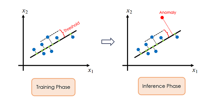
Traditionally, anomaly detection is conducted in a purely data-driven fashion: first, a machine learning model is trained to learn the normal operating characteristics of the system, usually based on the system data collected under pure normal operations. Then, a measure of abnormality, a.k.a the anomaly score, is defined, and the score threshold for flagging anomalies is determined. Afterward, the trained machine learning model is put into production to accept new data, and the model constantly calculates the anomaly scores for individual new data points as they come in. The data points with anomaly scores higher than the threshold will be identified as anomalies and subjected to later investigation.

Compared to the conventional data-driven paradigm, PINNs offer a new perspective for anomaly detection: besides fulfilling the data pattern, PINNs also check the physical consistency of the data to make the detection decision. By doing so, we can potentially reduce false positives, thus enhancing the reliability of the anomaly detection process.

📋 Case study

Zideh et al. [Physics-Informed Convolutional Autoencoder for Cyber Anomaly Detection in Power Distribution Grids] considered a cyber attack detection application for power distribution grids. Here, the authors assumed that the attacker may tamper with the system measurements to dysfunction the controller, and the goal is to determine if the data received by the controller is legitimate.

The prior work in anomaly detection in power distribution grids usually involves building autoencoder-based models. Like traditional PCA (shown in Figure 15), those autoencoder models are trained on normal operation data and they are learned to reconstruct those data. During inference, if the incoming data is anomalous, the autoencoder model will not be able to reconstruct it properly, leading to significant reconstruction errors and therefore large anomaly scores.

The novelty of this work lies in that the authors also considered physical inconsistency in addition to the data pattern as the criteria for detecting anomalies. Specifically, they trained a PINN-Autoencoder such that the reconstructed outputs (i.e., voltage and current magnitudes, phase angles, active/reactive power measurements) not only match with the given inputs, but also satisfy Kirchhoff's law, which encodes the physics-based relationships between measurements for power flow calculations. Consequently, during inference, even if the data pattern appears normal, any deviations from Kirchhoff's law would also signal a potential anomaly.

In their experiments, the authors claimed that their dual-check approach, which combines data pattern recognition with physical law validation, significantly enhanced the robustness and accuracy of the anomaly detection.

5.3 Health monitoring

Generally speaking, system health monitoring refers to the practice of continuous tracking and assessing the system's condition to detect signs of deterioration or failure. This is obviously an important task in practice to ensure the smooth operation of the system.

Compared to anomaly detection which assumes data is available and focuses on applying algorithms to identify unusual patterns, health monitoring emphasizes more on getting that system health data first, i.e., it targets the system observability.

In practice, however, we often encounter the challenge that the most critical indicators of a system's health are not directly measurable. As a result, we usually rely on indirect measurements and sophisticated models to infer the true health state of the system. This opens the door for employing PINNs.

More specifically, we can reformulate our health monitoring problem as a real-time parameter estimation problem, where we continuously estimate the values of those key health indicators based on the incoming (accessible) measurements. In the context of PINN, we can achieve that goal by optimizing the health indicators alongside the network's weights and biases, such that the predicted outcomes from PINN can be both data-consistent and physically plausible.

📋 Case study

Nath et al. [Physics-informed neural networks for predicting gas flow dynamics and unknown parameters in diesel engines] investigated the case of monitoring the health of diesel engines, where the key health indicators (e.g., heat transfer coefficient of the exhaust pipe) are difficult to measure directly.

To address this issue, the authors configured a PINN with those key health indicators as trainable parameters, which are optimized jointly with the neural network parameters to minimize physical and data losses. Once the training is completed, the values of the key health indicators that correspond to the measured field data will be obtained automatically. Afterward, those values can be used to infer the health of the engine.

5.4 Predictive maintenance

In practice, regular maintenance of the system is necessary to ensure optimal system operation. Over the years, the maintenance strategy gradually shifted from reactive (i.e., fixing the system after it fails) to proactive (i.e., anticipating when failures may occur and scheduling the maintenance activities accordingly), thanks to the advancements in both physical models for simulating failure mechanisms and algorithms for data analytics. This proactive way of performing maintenance gives rise to the term predictive maintenance.

In predictive maintenance, the main theme is to predict the evolution of the system health indicator and determine how long time remains until its value passes the pre-defined failure threshold. This time is generally referred to as remaining useful life (RUL) and constitutes one of the core indices to compute in predictive maintenance applications.

In practical implementations, however, a common challenge often faced by practitioners is that purely relying on either physical models or data models cannot deliver satisfactory results:

• For a purely physics-driven approach, the physics-based failure model generally contains coefficients that describe the unique conditions of the system at hand. Without knowing precisely the values of those coefficients, it is impossible to make reliable predictions of system status using the physical models.
• For a purely data-driven approach, the machine learning models trained on historical data cannot accurately extrapolate to failure cases they have never seen before. Since those data-driven models did not understand the underlying physical principles that govern the system's behavior, it is common that their predictions are statistically correct but physically implausible.

PINNs stand as a promising solution to overcome the above-mentioned limitations: as a physics-informed method, PINNs can natively incorporate the physical laws, thus enabling the model to produce physically consistent predictions even when extrapolating to unseen conditions. At the same time, as a data-driven approach, PINNs can effectively estimate those unknown system coefficients from the measurement data, therefore ensuring the models are tailored to the specific system at hand and promoting overall prediction accuracy.

📋 Case study

Wen et al. [Physics-Informed Neural Networks for Prognostics and Health Management of Lithium-Ion Batteries] applied PINNs to estimate the remaining useful life of Lithium-Ion batteries.

In their work, the authors developed a PINN to predict the evolution of the battery's capacity based on a semi-empirical PDE that governs the capacity degradation dynamics. Meanwhile, the measured battery capacity data was also used for PINN training to calibrate the unknown coefficients embedded in the empirical PDE. This empowers the model to deliver accurate predictions even in extrapolation scenarios.

For a battery, the remaining useful life is defined as the time when its currently usable capacity drops below a pre-specified threshold. By using the trained PINN to forecast the capacity trajectory, the authors could estimate when the battery will fail. This information is crucial for practical prognostics and health management of the Lithium-Ion battery.

5.5 Summary

In this section, we discussed PINN's applications in the scope of promoting a reliable and efficient operation of the system:

• Sensing: PINNs can provide accurate and efficient predictions of the system states. By complementing the field measurements, PINNs can greatly enhance the data quantity and quality for better system observability.
• Monitoring: PINNs can infer in real time the values of system health indicators from the sparse observational data, thus facilitating tracking and assessing the system's condition to detect signs of deterioration or failure.
• Diagnosing: PINNs can also serve as an anomaly detector to examine if the system displays unusual behaviors that deviate from the norm. Compared to the traditional anomaly detection strategies that only assess the data pattern consistency, PINNs additionally assess the physics consistency of the data, thus improving the robustness and accuracy of the anomaly detection.
• Forecasting: By fusing physical principles with observational data, PINNs can accurately model the system degradation process and estimate the system's remaining useful life until failure, thus enabling effective predictive maintenance.

Overall, from improving data quality and system observability to enabling robust anomaly detection and predictive maintenance, we can see the versatile role of PINNs in enhancing system operation.

6. Conclusion

In this blog, we went through common PINN application patterns developed by practitioners from various domains:

• Predictive modeling and simulations, where PINNs are leveraged for dynamical system forecasting, coupled system modeling, and surrogate modeling.
• Optimization, where PINNs are commonly employed to achieve efficient design optimization, inverse design, model predictive control, and optimized sensor placement.
• Data-driven insights, where PINNs are used to identify the unknown parameters or functional forms of the system, as well as to assimilate observational data to better estimate the system states.
• Data-driven enhancement, where PINNs are used to reconstruct the field and enhance the resolution of the observational data.
• Monitoring, diagnostic, and health assessment, where PINNs are leveraged to act as virtual sensors, anomaly detectors, health monitors, and predictive maintainers.

Overall, we see the versatility of the PINN methodology and its wide applications for different types of problems across various industries. There is no doubt that as the PINN technology keeps advancing, the application list we discussed in this blog will grow further. Nevertheless, I hope this list could give you a good starting point to navigate this exciting field.

If you find my content useful, you could buy me a coffee here🤗 Thank you very much for your support!

If you would like to learn more of physics-informed learning, I invite you to check out the following blogs: Unraveling the Design Pattern of Physics-Informed Neural Networks, Operator Learning via Physics-Informed DeepONet: Let's Implement It From Scratch, Discovering Differential Equations with Physics-Informed Neural Networks and Symbolic Regression.

You can also subscribe to my newsletter or follow me on Medium.