If you've clicked on this article, you've likely heard about Adam, a name that has gained notable recognition in many winning Kaggle competitions. It's common to experiment with a few optimizers like SGD, Adagrad, Adam, or AdamW, but truly understanding their mechanics is a different story. By the end of this post, you'll be among the select few who not only know about Adam optimization but also understand how to leverage its power effectively.

By the way, in my previous post I described the math behind Stochastic Gradient Descent, if you missed it, I recommend reading it.

Index

· 1: Understanding the Basics ∘ 1.1: What is the Adam Optimizer? ∘ 1.2: The Mechanics of Adam

· 2. Adam's Algorithm Explained ∘ 2.1 The Mathematics Behind Adam ∘ 2.2 The Role of Adaptive Learning Rates

· 3. Adam in Practice ∘ 3.1 Recreating the Algorithm from Scratch in Python ∘ 3.2 Adam in TensorFlow

· 4. Advantages and Challenges ∘ 4.1 Why Opt for Adam? ∘ 4.2 Addressing Adam's Limitations

· Conclusion

· Bibliography

1: Understanding the Basics

1.1: What is the Adam Optimizer?

In machine learning, Adam (Adaptive Moment Estimation) stands out as a highly efficient optimization algorithm. It's designed to adjust the learning rates of each parameter.

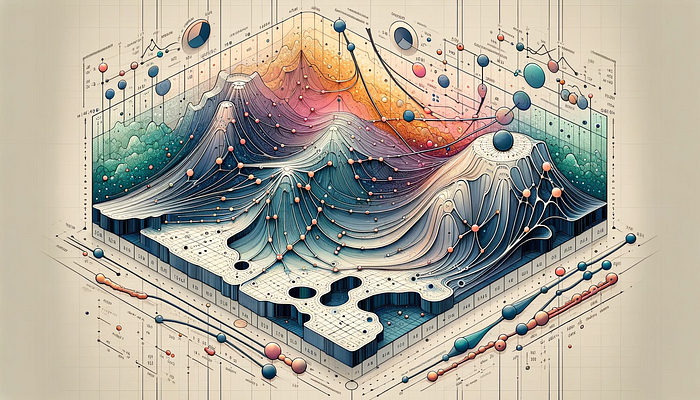
Imagine you're navigating a complex terrain, like the one in the image above. In some areas, you need to take large strides, while in others, cautious steps are required. Adam optimization works similarly, it dynamically adjusts its step size, making it larger in simpler regions and smaller in more complex ones, ensuring a more effective and quicker path to the lowest point, which represents the least loss in machine learning.

1.2: The Mechanics of Adam

Adam tweaks the gradient descent method by considering the moving average of the first and second-order moments of the gradient. This allows it to adapt the learning rates for each parameter intelligently.

At its core, Adam is designed to adapt to the characteristics of the data. It does this by maintaining individual learning rates for each parameter in your model. These rates are adjusted as the training progresses, based on the data it encounters.

Think of it as if you're driving a car over different terrains. In some places, you accelerate (when the path is clear and straight), and in others, you decelerate (when the path gets twisty or rough). Adam modifies its speed (the learning rate_ based on the road (the gradient's nature) ahead.

Indeed, the algorithm can remember the previous actions (gradients), and the new actions are guided by the previous ones. Therefore, Adams keeps track of the gradients from previous steps, allowing it to make informed adjustments to the parameters. This memory isn't just a simple average; it's a sophisticated combination of recent and past gradient information, giving more weight to the recent.

Moreover, in areas where the gradient (the slope of the loss function) changes rapidly or unpredictably, Adam takes smaller, more cautious steps. This helps avoid overshooting the minimum. Instead, in areas where the gradient changes slowly or predictably, it takes larger steps. This adaptability is key to Adam's efficiency, as it navigates the loss landscape more intelligently than algorithms with a fixed step size.

This adaptability makes Adam particularly useful in scenarios where the data or the function being optimized is complex or has noisy gradients.

2. Adam's Algorithm Explained

2.1 The Mathematics Behind Adam

As you may have understood, the core of Adam's algorithm lies in its computation of adaptive learning rates for each parameter.

1. Initialization In the beginning, Adam initializes two vectors, m, and v, which are both of the same shape as the parameters θ of the model. The vector m is intended to store the moving average of the gradients, while v keeps track of the moving average of the squared gradients. These moving averages are key to Adam's adaptive adjustments. A time step counter t is also initialized to zero. It keeps track of the number of iterations (or updates) that the algorithm has completed.

The initial values are typically set as follows:

• m0​=0 (Initial first-moment vector)
• v0​=0 (Initial second-moment vector)
• t=0 (Time step)

2. Compute Gradients For each iteration t, Adam computes the gradient gt​. This gradient is the derivative of the objective function (which we are trying to minimize) concerning the current model parameters θt​. Therefore, it represents the direction in which the function increases most rapidly.

Mathematically:

Where:

• gt​ represents the gradient at iteration t.
• ∇θ​ denotes the gradient for the parameters θ.
• ft​(θt−1​) is the objective function being optimized, evaluated at the parameter values from the previous iteration θt−1​.

3. Update m (first moment estimate) Then, we update the first-moment vector m, which stores the moving average of the gradients. This update is a combination of the previous value of m and the new gradient, weighted by parameters β1​ and 1−β1​, respectively. This process can be likened to having a short-term memory of past gradients, emphasizing more recent observations. It provides a smoothed estimate of the gradient direction.

Mathematically:

Where:

• mt​ is the first-moment vector at time step t.
• β1​ is the exponential decay rate for the first moment estimates (commonly set to around 0.9).
• gt​ is the gradient at time step t.

4. Update v (second raw moment estimate) Similarly, the second-moment vector v is updated. This vector gives an estimate of the variance (or unpredictability) of the gradients, therefore it stores the squared gradients that are accumulated. Like the first moment, this is also a weighted combination, but of the past squared gradients and the current squared gradient.

Mathematically:

Where:

• vt​ is the second-moment vector at time step t.
• β2​ is the exponential decay rate for the second-moment estimates (commonly set to around 0.999).

5. Correct the bias in the moments Since m and v are initialized to 0, they are biased toward 0, which leads to a bias towards zero, especially during the initial time steps, particularly during the initial steps. Adam overcomes this bias by correcting the vector by the decay rate, which is b1 for m (first-moment decay rate), and b2 for v (second-moment decay rate). This correction is important as it ensures that the moving averages are more representative, particularly in the early stages of training.

Mathematically:

Where:

• mt is the vector first-moment vector storing the moving average of the gradients at iteration t
• b1 is the decay rate of m at time t

Where​​:

• vt is the vector second-moment vector storing the variance of the gradients at iteration t
• b2 is the decay rate of vat time t

6. Update the parameters The final step is the update of the model parameters. This step is where the actual optimization takes place, moving the parameters in the direction that minimizes the loss function. The update utilizes the adaptive learning rates calculated in the previous steps.

Mathematically:

Where:

• θt+1​ represents the parameters after the update.
• θt​ represents the current parameters before the update.
• α is the learning rate, a crucial hyperparameter that determines the size of the step taken toward the minimum of the loss function.
• m^t​ is the bias-corrected first moment (mean) estimate of the gradients.
• v^t​ is the bias-corrected second moment (uncentered variance) estimate of the gradients.
• ϵ (epsilon) is a small scalar (e.g., 10^-8) added to prevent division by zero and maintain numerical stability.

2.2 The Role of Adaptive Learning Rates

The key feature of Adam is its adaptive learning rates. Unlike traditional gradient descent, where a single learning rate is applied to all parameters, Adam adjusts the rate based on how frequently a parameter is updated.

Like in other optimization algorithms, the learning rate is a critical factor in how significantly the model parameters are adjusted. A higher learning rate could lead to faster convergence but risks overshooting the minimum, while a lower learning rate ensures more stable convergence but at the risk of getting stuck in local minima or taking too long to converge.

The unique aspect of Adam is that the update to each parameter is scaled individually. The amount by which each parameter is adjusted is influenced by both the first moment (capturing the momentum of the gradients) and the second moment (reflecting the variability of the gradients). This adaptive adjustment leads to more efficient and effective optimization, especially in complex models with many parameters.

The small constant ϵ is added to prevent any issues with division by zero, which is especially important when the second moment estimate v^t​ is very small. This addition is a standard practice in numerical algorithms to ensure stability.

3. Adam in Practice

3.1 Recreating the Algorithm from Scratch in Python

Now let's move to the Python code, which really can make us understand how the algorithm works. In this example, I am recreating a simplified version of Adam, applied to Linear Regression. While, Adam is more commonly seen in the deep learning domain, building from scratch a Neural Network would require another post itself (follow me to stay updated, it's coming…). However, consider that you could replace the Linear Regression with other algorithms, as long as you adapt the code for it.

Let's get started with creating the AdamOptimizer class first:

# Adam Optimizer (use the class from the previous response)
class AdamOptimizer:
    def __init__(self, learning_rate=0.001, beta1=0.9, beta2=0.999, epsilon=1e-8):
        """
        Constructor for the AdamOptimizer class.

        Parameters
        ----------
        learning_rate : float
            Learning rate for the optimizer.
        beta1 : float
            Exponential decay rate for the first moment estimates.
        beta2 : float
            Exponential decay rate for the second moment estimates.
        epsilon : float
            Small value to prevent division by zero.

        Returns
        -------
        None.
        """
        self.learning_rate = learning_rate
        self.beta1 = beta1
        self.beta2 = beta2
        self.epsilon = epsilon
        self.m = None
        self.v = None
        self.t = 0

    def initialize_moments(self, params):
        """
        Initializes the first and second moment estimates.

        Parameters
        ----------
        params : dict
            Dictionary containing the model parameters.
        
        Returns
        -------
        None.
        """
        self.m = {k: np.zeros_like(v) for k, v in params.items()}
        self.v = {k: np.zeros_like(v) for k, v in params.items()}

    def update_params(self, params, grads):
        """
        Updates the model parameters using the Adam optimizer.

        Parameters
        ----------
        params : dict
            Dictionary containing the model parameters.
        grads : dict
            Dictionary containing the gradients for each parameter.
        
        Returns
        -------
        updated_params : dict
            Dictionary containing the updated model parameters.
        """
        if self.m is None or self.v is None:
            self.initialize_moments(params)

        self.t += 1
        updated_params = {}

        for key in params.keys():
            self.m[key] = self.beta1 * self.m[key] + (1 - self.beta1) * grads[key]
            self.v[key] = self.beta2 * self.v[key] + (1 - self.beta2) * np.square(grads[key])

            m_corrected = self.m[key] / (1 - self.beta1 ** self.t)
            v_corrected = self.v[key] / (1 - self.beta2 ** self.t)

            updated_params[key] = params[key] - self.learning_rate * m_corrected / (np.sqrt(v_corrected) + self.epsilon)

        return updated_params

The code can be broken down into three parts:

Initialization of the class

def __init__(self, learning_rate=0.001, beta1=0.9, beta2=0.999, epsilon=1e-8):
        self.learning_rate = learning_rate
        self.beta1 = beta1
        self.beta2 = beta2
        self.epsilon = epsilon
        self.m = None
        self.v = None
        self.t = 0

Here, the class requests as inputs the learning rate, beta 1 (first-moment decay rate), beta 2 (second-moment decay rate), and epsilon. Moreover, it temporarily sets the constants m, and v to None.

Initialization of the moment vectors

def initialize_moments(self, params):
        self.m = {k: np.zeros_like(v) for k, v in params.items()}
        self.v = {k: np.zeros_like(v) for k, v in params.items()}

In this step, we request an input "params", a dictionary storing the model parameters. In the linear regression case, the model parameters are weight and bias, therefore we will expect two keys.

Then, we initialize two dictionaries: m, the first-moment vector, which will store the moving average of the gradients, and v, the second-moment vector, which will store the variance of the gradients.

Both of them will have several keys equal to the number of keys in the params dictionary (in our case two), and each key will have a value array with the same length as the values in the original key in params. In this case, the value array will store only 0 values, as we are initializing it.

Update the params dictionary

def update_params(self, params, grads):
        if self.m is None or self.v is None:
            self.initialize_moments(params)

        self.t += 1
        updated_params = {}

        for key in params.keys():
            self.m[key] = self.beta1 * self.m[key] + (1 - self.beta1) * grads[key]
            self.v[key] = self.beta2 * self.v[key] + (1 - self.beta2) * np.square(grads[key])

            m_corrected = self.m[key] / (1 - self.beta1 ** self.t)
            v_corrected = self.v[key] / (1 - self.beta2 ** self.t)

            updated_params[key] = params[key] - self.learning_rate * m_corrected / (np.sqrt(v_corrected) + self.epsilon)

        return updated_params

The last step is the core of the AdamOptimizer class, it will first start by initializing the first and second-moment vectors if they are not initialized.

Then, we update self.t, which is the time counter, which was originally set to 0, when we initialized the class. We, then create an empty updated_params dictionary, that will store the new model parameters after Adam optimization.

Lastly, we run the Adam optimization algorithm on the existing parameters, by iterating over every parameter with a for a loop. Since this is the main aspect of our operation let's break it down:

self.m[key] = self.beta1 * self.m[key] + (1 - self.beta1) * grads[key]
self.v[key] = self.beta2 * self.v[key] + (1 - self.beta2) * np.square(grads[key])

These two lines of code update the first and second-moment vectors, using the formulas defined in subsection 2.1.

m_corrected = self.m[key] / (1 - self.beta1 ** self.t)
v_corrected = self.v[key] / (1 - self.beta2 ** self.t)

Here, we are updating the value in the two vectors by correcting them for the bias.

updated_params[key] = params[key] - self.learning_rate * m_corrected / (np.sqrt(v_corrected) + self.epsilon)

Lastly, we compute Adam optimization and store the new value in the updated_params dictionary.

Now, while this is technically the whole code we need for the Adam optimizer, this would be quite useless if we don't have anything to optimize. Therefore, we will create a Linear Regression class to feed something to Adam.

# Linear Regression Model
class LinearRegression:
    def __init__(self, n_features):
        """
        Constructor for the LinearRegression class.

        Parameters
        ----------
        n_features : int
            Number of features in the input data.
        
        Returns
        -------
        None.
        """
        self.weights = np.random.randn(n_features)
        self.bias = np.random.randn()

    def predict(self, X):
        """
        Predicts the target variable given the input data.

        Parameters
        ----------
        X : numpy array
            Input data.

        Returns
        -------
        numpy array
            Predictions.
        """
        return np.dot(X, self.weights) + self.bias

This code is pretty self-explanatory. However, suppose you want to know more about Linear Regression and call yourself a Linear Regression master. In that case, I highly recommend you to read my article about it, where I recreate a more complex version of the one defined above.

Lastly, we define a wrapper class, which will combine both the Adam Optimizer class and the Linear Regression class:

class ModelTrainer:
    def __init__(self, model, optimizer, n_epochs):
        """
        Constructor for the ModelTrainer class.

        Parameters
        ----------
        model : object
            Model to be trained.
        optimizer : object
            Optimizer to be used for training.
        n_epochs : int
            Number of training epochs.

        Returns
        -------
        None.
        """
        self.model = model
        self.optimizer = optimizer
        self.n_epochs = n_epochs

    def compute_gradients(self, X, y):
        """
        Computes the gradients of the mean squared error loss function
        with respect to the model parameters.

        Parameters
        ----------
        X : numpy array
            Input data.
        y : numpy array
            Target variable.
        
        Returns
        -------
        dict
            Dictionary containing the gradients for each parameter.
        """
        predictions = self.model.predict(X)
        errors = predictions - y
        dW = 2 * np.dot(X.T, errors) / len(y)
        db = 2 * np.mean(errors)
        return {'weights': dW, 'bias': db}

    def train(self, X, y, verbose=False):
        """
        Runs the training loop, updating the model parameters and optionally printing the loss.

        Parameters
        ----------
        X : numpy array
            Input data.
        y : numpy array
            Target variable.
        
        Returns
        -------
        None.
        """
        for epoch in range(self.n_epochs):
            grads = self.compute_gradients(X, y)
            params = {'weights': self.model.weights, 'bias': self.model.bias}
            updated_params = self.optimizer.update_params(params, grads)

            self.model.weights = updated_params['weights']
            self.model.bias = updated_params['bias']

            # Optionally, print loss here to observe training
            loss = np.mean((self.model.predict(X) - y) ** 2)
            if epoch % 1000 == 0 and verbose:
                print(f"Epoch {epoch}, Loss: {loss}")

The main goal of the class is to iterate for several iterations given by the variable n_epochs optimizing the parameters of the linear regression by the Adam optimizer.

Compute the gradients

def compute_gradients(self, X, y):
        predictions = self.model.predict(X)
        errors = predictions - y
        dW = 2 * np.dot(X.T, errors) / len(y)
        db = 2 * np.mean(errors)
        return {'weights': dW, 'bias': db}

In this class, we finally compute the gradients. Indeed, in Subsection 2.1 that was the second step. Here it was not possible to calculate the gradients until we defined a model. Therefore, this function will vary based on the model you will feed to Adam. Since we are using Linear regression we only need to calculate the gradient of the weights and the bias.

Train

def train(self, X, y, verbose=False):
        for epoch in range(self.n_epochs):
            grads = self.compute_gradients(X, y)
            params = {'weights': self.model.weights, 'bias': self.model.bias}
            updated_params = self.optimizer.update_params(params, grads)

            self.model.weights = updated_params['weights']
            self.model.bias = updated_params['bias']

            loss = np.mean((self.model.predict(X) - y) ** 2)
            if epoch % 1000 == 0 and verbose:
                print(f"Epoch {epoch}, Loss: {loss}")

Finally, we create the train method. As we mentioned before, this class iterates n_epochs times. In each iteration, it computes the gradients of weights and bias resulting from Linear Regression, then feeds the gradients to the Adam optimizers, and sets the resulting weights and bias back to the model.

You can access the complete code with its implementation in a Jupyter Notebook here:

3.2 Adam in TensorFlow

At this point, you will have a good understanding of the Adam optimizer. Now that you know how it works, you actually can discard the code above as you'll likely use a more efficient implementation from Tensorflow or PyTorch with just a few lines of code.

In this case, we will use TensorFlow, and we will create a simple neural network with two layers and 64 nodes. Then, we will "compile" the model with Adam optimization. While compiling the optimizer is adjusting the weights of the network to minimize the loss.

import tensorflow as tf
import numpy as np

# Generate Sample Data
# For demonstration, we create synthetic data for a regression task
X = np.random.rand(100, 3)  # 100 samples, 3 features
y = X @ np.array([2.0, -1.0, 3.0]) + 1.5  # Linear relationship with some coefficients and bias

# Create the Neural Network
model = tf.keras.Sequential([
    tf.keras.layers.Dense(64, activation='relu', input_shape=(3,)),  # Input layer with 3 inputs
    tf.keras.layers.Dense(64, activation='relu'),  # Another dense layer
    tf.keras.layers.Dense(1)  # Output layer with 1 unit (for regression)
])

# Compile the Model with the Adam Optimizer
model.compile(optimizer=tf.keras.optimizers.Adam(learning_rate=0.001),
              loss='mean_squared_error')  # MSE is typical for regression

# Train the Model
model.fit(X, y, epochs=10)  # Train for 10 epochs as an example

4. Advantages and Challenges

4.1 Why Opt for Adam?

At this point, you know how the algorithm works, but you may still wondering when is Adam a good choice.

1. Dealing with Sparse Data Adam is particularly effective when working with data that leads to sparse gradients. This situation is common in models with large embedding layers or when dealing with text data in natural language processing tasks.

2. Training Large-Scale Models Adam is well-suited for training models with a large number of parameters, such as deep neural networks. Its adaptive learning rate helps navigate the complex optimization landscapes of such models efficiently. However, this is not always the case, as we can see when we applied Adam to Linear Regression.

3. Achieving Rapid Convergence When we don't have much time for the convergence to happen, Adam comes to help. This is thanks to its adaptive learning, which guarantees a faster convergence compared to its rival SGD.

4. For Online and Batch Training It's versatile enough to be used in both online learning scenarios (where the model is updated continuously as new data arrives) and batch learning.

4.2 Addressing Adam's Limitations

While the Adam optimizer is versatile and effective in many scenarios, there are certain challenges and considerations to keep in mind.

1. Tuning Hyperparameters While Adam is less sensitive to learning rate changes compared to other optimizers, choosing an appropriate initial learning rate is still crucial. A too-high learning rate may lead to instability, while too low a rate can slow down the training process. The default values of β1​ and β2​ (typically 0.9 and 0.999, respectively) work well in most cases, but in some scenarios, adjusting them can yield better results.

2. Handling Noisy Data and Outliers While Adam is generally robust to noisy data, extreme outliers or highly noisy datasets might impact its performance. Preprocessing data to remove or diminish the impact of outliers can be beneficial.

3. Choice of Loss Function The efficiency of Adam can vary with different loss functions. Make sure that the loss function resonates with the problem you are solving, and experiment with a few of them to see which one works best.

4. Computational Considerations Adam typically requires more memory than simple gradient descent algorithms because it maintains moving averages for each parameter. This should be considered when working with very large models or limited computational resources.

Conclusion

To effectively leverage Adam, it's essential to understand both its strengths and limitations. Fine-tuning its parameters and being mindful of the nature of your data and problem can help in harnessing its full potential. Regular monitoring and validation are key to ensuring that the optimizer is performing optimally. Keep in mind these challenges, follow the best practices recommended in this article and you are ready to experiment with Adam.

Bibliography

1. Kingma, D. P., & Ba, J. (2014). Adam: A method for stochastic optimization. arXiv preprint arXiv:1412.6980. https://arxiv.org/abs/1412.6980
2. Ruder, S. (2016). An overview of gradient descent optimization algorithms. arXiv preprint arXiv:1609.04747. https://arxiv.org/abs/1609.04747
3. Goodfellow, I., Bengio, Y., & Courville, A. (2016). Deep Learning. MIT Press. http://www.deeplearningbook.org/

If you liked this article consider leaving a like, and follow me to be updated on my latest posts. My goal is to recreate all the most popular algorithms from scratch and make machine learning accessible to everyone.