Transform semantic point clouds into intelligent OpenUSD scene graphs with spatial relationships. Complete Python tutorial with NetworkX and LLM integration.

The hardest part of spatial AI isn't the algorithms.

It's making 3D data understandable for you, me, and the people who could really benefit from the knowledge (perhaps one of them is the grandmother next door).

When prototyping with Python, we geekily get satisfaction from visualizing colored point clouds. It is a nice sight!

But it may not be very useful for others or decision-making applications.

Indeed, your 3D data contains relationships, hierarchies, and semantic meaning that the point cloud formats can't capture.

And we need to leverage that to open the door to queryable spatial intelligence.

To enable autonomous systems to understand 3D environments like humans do.

And this is why we propose exploring an innovative idea:

What if we simply recognized each "object" in the point cloud, labeled it with a word that best describes it, and then generated relationships between the scene constituents?

The result would be a scene graph with semantic relationships!

🎵 Note to Readers: This hands-on guide is part of a UTWENTE joint work with co-authors F. Poux and V. Lehtola.

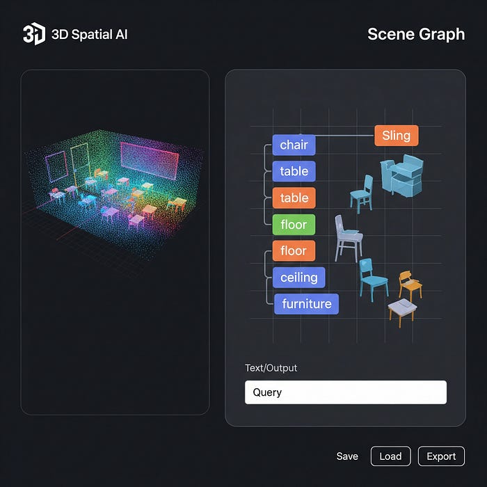
We could then use it to unlock natural language queries through LLMs integration, and create an innovation like this one:

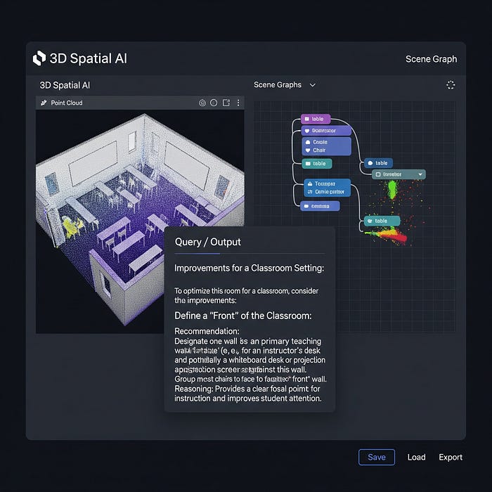
It could enable spatial agents to answer queries such as "find all chairs positioned for conversation"

or "identify cluttered areas blocking wheelchair access,"

Making 3D data actionable for both human operators and AI systems.

This tutorial shows you how to extract that intelligence, visualize it, and encode it into production-ready OpenUSD scenes.

🐦 Ville's Note: From scans and point clouds, digital applications require the processing of either Building Information Models (BIM) or Universal Scene Descriptions (USD).

🦚 Florent's Note: OpenUSD provides an industry-standard framework capable of encoding these relationships. Originally developed by Pixar for animation pipelines, USD has evolved into the universal language for 3D scene description across industries from film to robotics, and is pushed by NVIDIA.

From there, we will test various Spatial-aware LLMs to determine if we have created an AI-ready system (the access to materials + code + bonus resources is shared at the end of the end of the article).

If you are ready, let us unlock a massive new set of skills and level up!

🦚 Florent Poux, Ph.D.: If you are new to my (3D) writing world, welcome! We are going on an exciting adventure that will allow you to master an essential 3D Python skill. Before diving, I like to establish a clear scenario, the mission brief.

Once the scene is laid out, we embark on the Python journey. Everything is given. You will see Tips (Growing Notes and Geeky Notes), the code (Python), and diagrams to help you get the most out of this article. Thanks to the 3D Geodata Academy and UTWENTE for their support of this endeavor.

Your Mission: Transform Static Point Clouds Into Intelligent Spatial Understanding

You've been hired by a robotics company to develop the next generation of autonomous robots, by using LIDAR data for teaching.

These aren't simple rule-following machines. They need to understand contexts, including complex 3D environments, like humans do.

Picture the classroom: tables, scattered chairs, moving furniture, students navigating narrow aisles. Your robot needs to answer questions that go far beyond basic navigation:

• "Which packages are stacked and safe to pick?"
• "What's the clearest path to the loading dock?"
• "Are there any unstable storage configurations?"
• "Which areas are too cluttered for safe operation?"

You start investigating the current 3D Tech, and your first insight is that the (colored) point cloud is not an answer to any of these questions, as it just contains millions of coordinates. And coordinates don't answer these questions.

Traditional point cloud processing gives you millions of coordinates. But coordinates don't answer these questions. Spatial relationships do.

This means that you are going to avoid treating point clouds as geometry. You'll transform them into knowledge. Knowledge that can be queried, organized, and reorganized, which has similarities to how humans think.

And this also means encoding everything into industry-standard formats that production systems understand. Your spatial intelligence doesn't stay trapped in research code. It must become the brain of real autonomous systems.

You'll know you've succeeded when:

• Your teaching robots navigate complex environments with human-like spatial understanding
• Users query your system in natural language and get precise spatial answers
• Your spatial intelligence integrates seamlessly with existing production workflows
• Other developers study your approach as the new standard for 3D scene understanding

Okay, you now have a clear direction, with an objective. Let us detail the workflow.

The Workflow: From Point Cloud to Scene Graph

Building intelligent scene representations requires a systematic approach.

The transformation from raw point cloud data to structured USD scenes follows a clear pipeline. Each stage adds a layer of understanding, progressing from geometry to semantics to relationships.

Your workflow begins with semantic point cloud data — coordinates enriched with classification labels.

🦚 Florent's Note: I detail in Step 1 how to generate such a semantic point cloud with manual, hybrid, or fully automatic approaches.

The pipeline then extracts individual objects through clustering, computes spatial relationships, and finally encodes everything into OpenUSD format.

The system design prioritizes modularity and extensibility.

Each processing stage operates independently, allowing you to customize algorithms without breaking the pipeline.

This architecture scales from single rooms to entire building complexes.

🦥 Florent's Geeky Note: The pipeline uses NetworkX for graph operations and OpenUSD for scene encoding. DBSCAN clustering parameters (eps=0.8, min_samples=15) work well for room-scale scenes but may need adjustment for other scales.

🐦 Ville's Note: Geeky notes are my favorite!

By the end of this journey, you'll have constructed a complete spatial intelligence pipeline:

• Input: Raw LiDAR scans (the semantic injection is shown in complimentary tutorials)
• Processing: Instance object detection (leveraging DBSCAN Clustering), spatial relationship extraction, scene graph construction (Networkx and Graph Theory).
• Output: Intelligent USD scenes that answer complex spatial queries (OpenUSD) and usable for LLM integration.

A Word on Scene Graphs in 3D Data Science

Scene graphs aren't just fancy data structures.

They're the missing link between raw geometry and intelligent spatial understanding.

🐦 Ville's Geeky Note: I cannot refrain from sharing some additional pointers. An ontology is the formal vocabulary and ruleset that constrains scene graphs. A scene graph is a case-specific set of nodes (words used as labels) and edges (relations) that should comply with that ontology. Large language models and their embedded knowledge can be harnessed (cautiously!) to suggest, check, or flag inconsistencies in a scene graph.

While traditional 3D formats store vertices and faces, scene graphs capture the relationships that make spaces meaningful.

Think about a room scan from your LiDAR sensor. You have millions of points labeled as "chair," "table," or "wall."

But what you really need to know is that the chair sits next to the table, the lamp is on the table, and the bookshelf is against the wall.

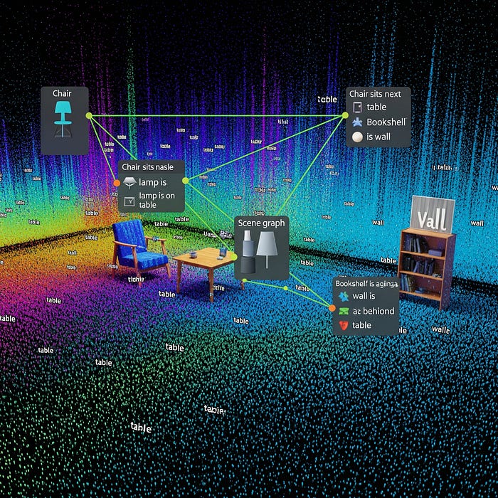
Scene graphs encode this spatial intelligence directly into your data structure.

Each object becomes a node with semantic properties, connected by edges that describe spatial relationships. This transforms passive geometry into queryable knowledge.

🌱 Florent's Note: Scene graphs excel in applications requiring spatial reasoning — from autonomous navigation to architectural analysis. The relationships you encode today become the queries you can answer tomorrow.

Initialization: Environment considerations

Let me assume you have Anaconda installed. If not, download and install the Anaconda Distribution for your operating system from anaconda.com/download.

[OPTIONAL] Python Setup from scratch

Open your Anaconda Prompt (Windows) or Terminal (macOS/Linux). This keeps your project dependencies isolated. then:

conda create -n my_data_env python=3.9

• my_data_env: Replace with your preferred environment name.
• python=3.9: Specify your desired Python version.

After that, you must activate the environment before installing packages into it.

conda activate my_data_env

Then, use pip for most packages as it handles dependencies well.

pip install numpy pandas networkx scikit-learn matplotlib

• json is a built-in Python module, so no installation is needed.
• scikit-learn includes DBSCAN.
• matplotlib.patches comes with matplotlib.

Then, install open3d via pip. Ensure your environment is still active.

pip install open3d

Finally, install an IDE such as Spyder directly into your new environment to ensure it uses the correct Python interpreter and libraries.

pip install spyder

With your environment still active, you can launch Spyder:

spyder

Spyder will now open, configured to use the my_data_env environment and all the libraries you've installed.

🐦 Ville's Note: You can verify the installed packages by running pip list or conda list in Spyder's IPython console, or by trying to import them in a new script.

This looks like a great introductory section for a tutorial! Here's a comment on each part, suitable for explaining to a user:

Loading Libraries in Python

To kick things off, the first step in any robust Python project is to gather our tools — our libraries!

We're importing the collection of powerful packages that will serve different purposes throughout our journey. To get started, we are going to load 7 libraries in our Python script:

#Base libraries
import numpy as np
import pandas as pd
import json

#Graph and algorithm-related libraries
import networkx as nx
from sklearn.cluster import DBSCAN

# For visualization
import open3d as o3d
import matplotlib.pyplot as plt
import matplotlib.patches as mpatches

And then, we isolate this to guide even more the installation of OpenUSD.

OpenUSD (Universal Scene Description) is a powerful framework for describing, composing, simulating, and collaborating on 3D scenes. Let us use it:

try:
    from pxr import Usd, UsdGeom, Sdf, Gf, UsdShade
    USD_AVAILABLE = True
except ImportError:
    print("USD not available. Install with: pip install usd-core")
    USD_AVAILABLE = False

This try-except block is a very elegant way to handle an optional dependency.

Now that our development environment is prepared with all the necessary tools, it's time to get our hands dirty!

To build the pipeline, we are going to go into this 12-step solution, as illustrated below.

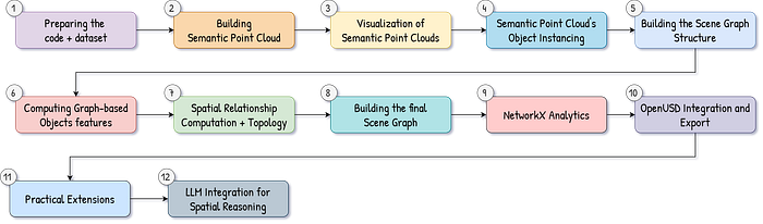
The next logical step is to load a 3D dataset, which will be the raw material for our analysis, graph construction, and visualization.

Step 1. Preparing a dataset

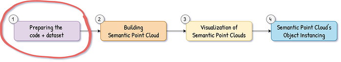
Semantic point clouds are your scene graph generation starting point.

Unlike raw point clouds that only contain coordinates and colors, semantic point clouds include object class labels for every point.

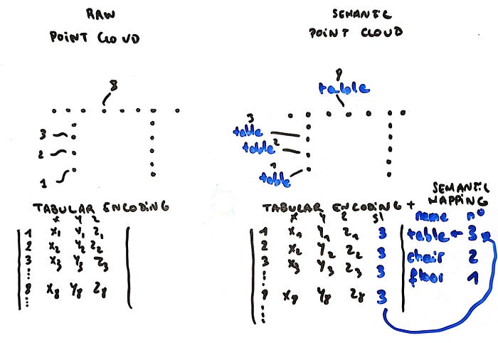
Each coordinate knows whether it belongs to a chair, table, wall, or floor.

The transformation happens in three stages: raw data acquisition, preprocessing and cleaning, and then semantic labeling.

Each stage has its own challenges and solutions that determine your final spatial intelligence quality.

Your input might be noisy LiDAR scans with billions of points. Your output needs to be clean, labeled coordinates ready for object extraction and relationship detection.

🌱 Florent's Note: The quality of your semantic labels directly impacts scene graph accuracy. Invest time in this preparation stage — it's the foundation of everything that follows. For the complete AI-assisted workflow, I highly encourage you to check out the course 3D Segmentor OS.

Semantic Labeling Strategies

Semantic labeling assigns object class labels to every point in your cloud.

This transformation from geometric coordinates to semantic understanding enables all downstream spatial intelligence extraction.

You have, in essence, three main approaches: manual annotation, automated classification, and hybrid workflows.

Each approach has different accuracy, speed, and scalability trade-offs that affect your project's feasibility and final quality.

Manual Annotation Workflows: Manual annotation provides the highest accuracy but requires significant human effort. Professional annotation tools streamline the process while maintaining quality control.

Manual annotation works best for small, high-value datasets where perfect accuracy is essential. Consider it for training data generation or critical scene validation.

🌱 Florent's Note: Start manual annotation with the largest, most obvious objects (floors, walls, ceilings). These provide context that makes smaller object annotations much faster and more accurate.

Automated Classification Pipelines: Automated semantic labeling uses machine learning models to classify points based on geometric and visual features.

Modern approaches combine traditional feature engineering with deep learning for robust performance.

You can find such a solution in this tutorial:

Automated labeling scales to large datasets but requires careful validation and often needs manual correction for complex scenes.

Hybrid Annotation Strategies: Hybrid approaches combine the best of manual and automated methods. Use automation for initial labeling, then apply targeted manual correction for critical areas or challenging classifications.

🦥 Ville's Geeky Note: Confidence thresholding at 0.8 typically catches 80–90% of classification errors while requiring manual review of only 10–20% of points. Adjust based on your accuracy requirements and annotation budget.

Hybrid workflows provide the scalability of automation with the accuracy of manual validation, making them ideal for production semantic labeling pipelines.

🌱 Growing Note: For getting a hands-on solution, you can check out the course Segmentor OS.

Validation and Quality Control

Semantic point cloud quality directly impacts scene graph accuracy.

Validation catches labeling errors before they propagate through your spatial intelligence pipeline. Three validation approaches ensure your semantic labels meet production requirements: geometric consistency checks, statistical quality metrics, and cross-validation with ground truth.

Quality control is not optional. Bad semantic labels create phantom objects, missing relationships, and unreliable spatial intelligence that breaks downstream applications.

Before using your semantic point cloud for scene graph generation, verify that it meets production standards:

Geometric Quality:

• ✅ Floor surfaces are horizontal (normal deviation < 0.1)
• ✅ Wall surfaces are vertical (horizontal normal component < 0.2)
• ✅ Furniture objects rest on supporting surfaces
• ✅ No floating objects without physical support

Semantic Quality:

• ✅ All points have valid semantic labels (coverage > 95%)
• ✅ Similar nearby points have consistent labels (coherence > 85%)
• ✅ Object boundaries are clean and well-defined
• ✅ No semantic fragmentation (single objects not split into multiple pieces)

Data Quality:

• ✅ Coordinate system properly aligned (Z-up, consistent scale)
• ✅ Point density normalized across the scene
• ✅ Noise and outliers removed
• ✅ File format compatible with downstream pipeline

Your semantic point cloud is now ready for scene graph generation. Clean geometry, accurate labels, and validated quality ensure that your spatial intelligence extraction will produce reliable, production-ready results.

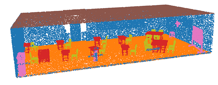
🦥 Florent's Geeky Note: I have prepared a dataset for you, which you can find at the end of the article if you don't have your own 3D data to work with. It is from a classroom with furniture.

Step 2. The Semantic Point Cloud in Python

Now that our environment's all set up, let's get to the heart of our tutorial: loading our 3D data.

We'll define a simple Python function to read a semantic point cloud from a CSV file. This function will not only load the raw data but also make it more human-readable by mapping numerical labels to meaningful class names.

Here's the function we'll use:

def load_semantic_point_cloud(file_path, column_name = 'semantic_label'):
    """Load semantic point cloud data from ASCII formats."""
        
    df = pd.read_csv(file_path, delimiter=';')
    class_names = ['ceiling', 'floor', 'wall', 'chair', 'furniture', 'table']
    
    # Assuming the numerical labels are 0.0, 1.0, 2.0, ...
    label_map = {float(i): class_names[i] for i in range(len(class_names))}
    
    df[column_name] = df[column_name].map(label_map)
    
    # I sample here for replication goals
    return df.sample(n=150000, random_state=1)

Now, let's call our function to load the data and then take a smaller sample for immediate visualization and demonstration:

# Let us control the output of
raw_data = load_semantic_point_cloud('../DATA/indoor_room_labelled.csv')
# I sample here for replication goals
demo_data = raw_data.sample(n=100000, random_state=1)

from there, let us look at what it looks like:

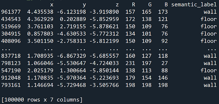
The load_semantic_point_cloud function, along with its subsequent sampling, is designed to give you a clean, manageable Pandas DataFrame containing your 3D point cloud data with human-readable labels.

Having demo_data in this well-structured and semantically labeled format means you're perfectly set up for the next steps in your tutorial.

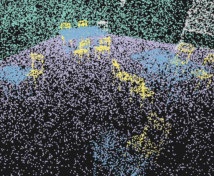
Step 3. The Visualization of Semantic Point Clouds

With our 3D point cloud loaded and neatly organized, it's time to bring it to life!

We'll use Open3D, our powerful 3D visualization library, to render the demo_data we prepared. This will give us our first real look at the room furniture and structure captured in the point cloud.

Here's the function designed to do just that:

def visualize_semantic_pointcloud(df, point_size = 2.0):
    """Visualize semantic point cloud with flat colors per semantic label using Open3D."""
    
    # Extract coordinates
    points = df[['x', 'y', 'z']].values
    
    # Create Open3D point cloud
    pcd = o3d.geometry.PointCloud()
    pcd.points = o3d.utility.Vector3dVector(points)
    
    # Create color mapping for semantic labels
    unique_labels = df['semantic_label'].unique()
    color_map = {}
    
    # Generate distinct colors for each label
    for i, label in enumerate(unique_labels):
        hue = i / len(unique_labels)
        color_map[label] = plt.cm.tab10(hue)[:3]
    
    # Assign colors based on semantic labels
    colors = np.array([color_map[label] for label in df['semantic_label']])
    pcd.colors = o3d.utility.Vector3dVector(colors)
    
    # Create visualization
    vis = o3d.visualization.Visualizer()
    vis.create_window(window_name="Semantic Point Cloud", width=1200, height=800)
    vis.add_geometry(pcd)
    
    # Set point size
    render_option = vis.get_render_option()
    render_option.point_size = point_size
    
    print(f"Visualizing {len(points)} points with {len(unique_labels)} semantic classes:")
    for label in unique_labels:
        count = (df['semantic_label'] == label).sum()
        print(f"  {label}: {count} points")
    
    vis.run()
    vis.destroy_window()

This function visualizes our 3D semantic point cloud by extracting coordinates and labels from a Pandas DataFrame, then creating an Open3D point cloud.

It intelligently assigns unique colors to each semantic class before setting up and launching an interactive Open3D viewer.

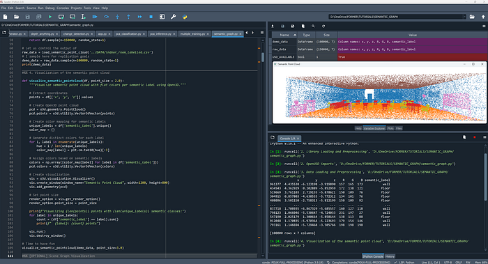
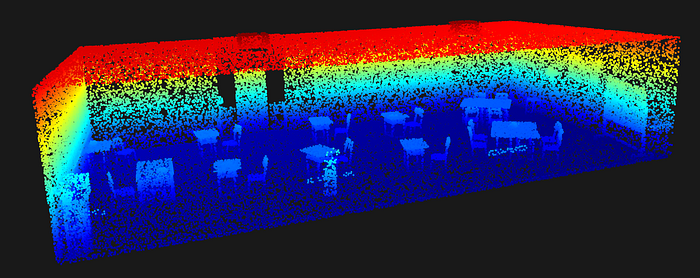
Now, let's execute our visualization function to see our demo_data in action:

# Time to have fun
visualize_semantic_pointcloud(demo_data, point_size=3.0)

By calling visualize_semantic_pointcloud(demo_data, point_size=3.0), we pass our smaller, sampled dataset to the function and set a slightly larger point_size of 3.0 to make the individual points a bit more prominent.

When you run this line, a new window will pop up, displaying your 3D room point cloud, with each semantic object clearly delineated by its assigned color.

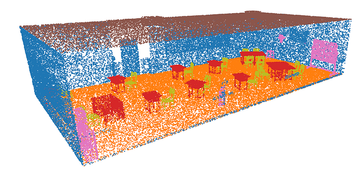
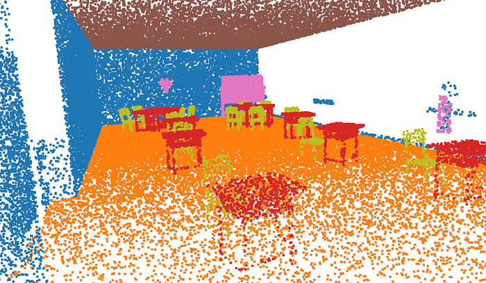
Beautiful. Now, let us try to adjust the granular nature of the semantic description.

Step 4. Semantic Point Cloud's Object Instancing

Raw point cloud data needs structure before it reveals meaning.

The preprocessing stage transforms unorganized coordinates into meaningful object clusters.

Your semantic point cloud arrives with labels like "chair" or "table," but those labels are scattered across thousands of individual points.

We want to create a function that takes this soup of points and finds distinct objects hiding in this.

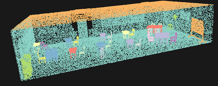
That's exactly what extract_semantic_objects() does. We want to hunt through our point cloud, semantic label by semantic label, and use DBSCAN clustering to find discrete objects.

🐦RVile's Note: DBSCAN clustering groups spatially connected points with identical semantic labels. This separates multiple chairs in a room and handles complex geometries better than simple bounding boxes.

We are going to work in three stages:

Step 1: We loop through each unique semantic label (chair, table, floor). It doesn't mix different object types. Smart move - you don't want chair points clustering with table points.

Step 2: Apply DBSCAN for each semantic class, where DBSCAN asks two questions:

• Are these points close enough to belong together? (controlled by eps)
• Are there enough points to form a real object? (controlled by min_samples)

Step 3: Each discovered object gets packaged with:

• All its constituent points
• Centroid position (the object's center of mass)
• Bounding box (min/max coordinates in each dimension)
• Point count (how much data supports this object)

This is all happening in this function:

def extract_semantic_objects(df: pd.DataFrame, eps: float = 0.5, min_samples: int = 10) -> Dict:
    """Extract individual objects from semantic point cloud using clustering."""
    objects = {}
    
    for label in df['semantic_label'].unique():
        label_points = df[df['semantic_label'] == label]
        
        if len(label_points) < min_samples:
            continue
            
        # Apply DBSCAN clustering
        coords = label_points[['x', 'y', 'z']].values
        clustering = DBSCAN(eps=eps, min_samples=min_samples).fit(coords)
        
        # Group by cluster
        label_points_copy = label_points.copy()
        label_points_copy['cluster'] = clustering.labels_
        
        for cluster_id in np.unique(clustering.labels_):
            if cluster_id == -1:  # Skip noise points
                continue
                
            cluster_points = label_points_copy[label_points_copy['cluster'] == cluster_id]
            object_key = f"{label}_{cluster_id}"
            
            objects[object_key] = {
                'points': cluster_points,
                'centroid': cluster_points[['x', 'y', 'z']].mean().values,
                'bounds': {
                    'min': cluster_points[['x', 'y', 'z']].min().values,
                    'max': cluster_points[['x', 'y', 'z']].max().values
                },
                'semantic_label': label,
                'point_count': len(cluster_points)
            }
    
    return objects

The algorithm handles edge cases gracefully. Small point clusters below the minimum threshold get filtered out as noise. This prevents spurious detections while preserving genuine objects.

Before moving onto next stages, let me highlight some key considerations about the parameters.

The eps parameter controls how close points need to be to belong together. Think of it as adjusting a magnifying glass.

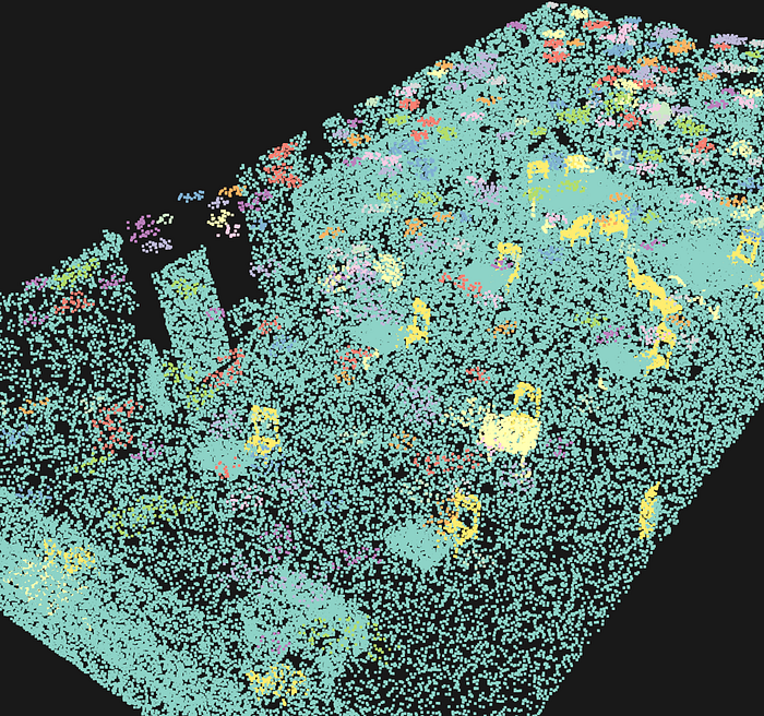
Too tight (eps = 0.1): Your chair splits into armrest, seat, and backrest. Three objects instead of one.

Just right (eps = 0.3): All chair points unite. One solid object emerges.

Too loose (eps = 3.0): Chair and nearby table merge. Spatial chaos returns.

Each extracted object includes essential geometric properties — centroid position, bounding box, and point density. These become the foundation for spatial relationship analysis in the next stage.

🦥 Florent's Geeky Note: The eps parameter controls clustering sensitivity — smaller values create more separate objects, larger values merge nearby items. Start with 0.5–1.0 for room-scale scenes and adjust based on your point cloud density. The optimal eps often equals 2–3 times your average point spacing. Dense LiDAR scans need smaller eps values than sparse smartphone captures. You can check out the book for a complete deep dive

Also, the min_sample parameter decides what counts as a real object.

⚠️ Ville's Warning: Setting min_samples too low creates spurious micro-objects from noise. Too high and you lose legitimate small objects like lamps or decorative items.

🌱 Growing Note: Start with min_samples = point_count/50 for each semantic class. Adjust based on your specific objects and scanning density.

This stage allows us to obtain a dictionary called objects, which holds all the necessary information for each object:

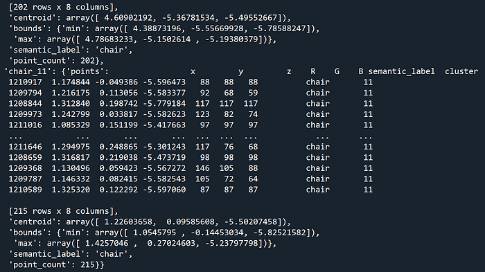
This is our starting point to build our scene graph!

Step 5. Building the Scene Graph Structure

Scene graphs transform isolated objects into connected knowledge.

The graph construction process creates nodes for each object and edges for spatial relationships.

To achieve this, we are going to leverage NetworkX.

let us import the library:

import networkx as nx
import matplotlib.pyplot as plt

NetworkX provides the graph infrastructure, while we are going to develop custom algorithms to determine relationship types based on geometric and topological analysis. Let us create a simple graph with the code below:

def visualize_room_furniture_graph(furniture_data):
    """Builds and visualizes a graph of room furniture."""
    
    G = nx.Graph()
    for item, connections in furniture_data.items():
        G.add_node(item)
        for connected_item in connections:
            G.add_edge(item, connected_item)
    pos = nx.spring_layout(G, seed=42)  # For reproducible layout
    nx.draw(G, pos, with_labels=True, node_color='salmon',
            node_size=500, font_size=10, font_weight='bold')
    plt.title("Room Furniture Graph")
    plt.show()
# Example of a room description:
room_layout = {
    "bed": ["nightstand", "lamp", "rug"],
    "nightstand": ["bed", "lamp"],
    "lamp": ["bed", "nightstand"],
    "rug": ["bed", "sofa", "bookshelf"],
    "sofa": ["coffee table", "TV", "rug"],
    "coffee table": ["sofa", "TV"],
    "TV": ["sofa", "coffee table", "TV stand"],
    "TV stand": ["TV"],
    "bookshelf": ["desk"],
    "desk": ["bookshelf", "chair"],
    "chair": ["desk"]
}
visualize_room_furniture_graph(room_layout)

As you can see, this allows us to interpret a dictionary, and turn that into a graph as shown below:

But for real scenes, we have 50+ objects with complex relationships.

For these cases, scene graphs need hierarchy, attributes, and spatial intelligence. Here is an example of a three-layer architecture that is very useful:

Layer 1: Scene Level

• Root node contains the entire scene
• Bounds, object counts, overall statistics

Layer 2: Semantic Groups

• Group all chairs together
• Group all tables together
• Enables semantic queries

Layer 3: Individual Objects

• Each detected object becomes a node
• Rich attributes for spatial reasoning

But first, let us focus on the nodes and compute the necessary object features.

Step 6. Computing Objects features

We have found objects, but we only know their basic coordinates and some geometric features.

Let us define a new function, compute_object_features(), to extract additional insight about each object's geometry and characteristics.

We will want to compute three categories of features to be as exhaustive as possible:

Geometric Properties:

• Volume (how much 3D space the object occupies)
• Surface area (the object's outer skin area)
• Compactness (how "sphere-like" vs elongated the object is)

Dimensional Analysis:

• Height (Z-dimension extent)
• Point density (how many points per unit volume)

Shape Characteristics:

• Bounding box analysis
• Spatial extent in each dimension

This will help us with future tasks. Let us start by computing the surface area.

Given a cloud of points on an object's surface, how much total surface area does the object have? It's like wrapping the object in shrink-wrap and measuring the wrap's area.

Uses the convex hull method — imagine stretching a rubber sheet around the object's outermost points. Not perfect for concave objects, but robust and fast.

def estimate_surface_area(points):
    from scipy.spatial import ConvexHull
    try:
        hull = ConvexHull(points)
        return hull.area  # Surface area of convex hull
    except:
        return 0.0  # Fallback for degenerate cases

Why Convex Hull?

• Fast computation even for thousands of points
• Always produces valid results (no self-intersections)
• Good approximation for most furniture objects
• Handles irregular point distributions gracefully

For highly concave objects (L-shaped desks, hollow objects), consider alpha shapes or Poisson surface reconstruction for more accurate area estimates.

🦥 Ville's Geeky Note: ConvexHull fails when points are coplanar (all in one plane) or collinear (all on one line). The try-except block catches these edge cases.

Now, let us create a function that computes all the features, including our surface area as defined above:

def compute_object_features(objects):
    """Compute geometric and semantic features for each object."""
    features = {}
    
    for obj_name, obj_data in objects.items():
        points = obj_data['points'][['x', 'y', 'z']].values
        
        # Geometric features
        volume = np.prod(obj_data['bounds']['max'] - obj_data['bounds']['min'])
        surface_area = estimate_surface_area(points)
        compactness = (surface_area ** 3) / (36 * np.pi * volume ** 2) if volume > 0 else 0
        
        features[obj_name] = {
            'volume': volume,
            'surface_area': surface_area,
            'compactness': compactness,
            'height': obj_data['bounds']['max'][2] - obj_data['bounds']['min'][2],
            'semantic_label': obj_data['semantic_label'],
            'centroid': obj_data['centroid'],
            'point_density': obj_data['point_count'] / volume if volume > 0 else 0
        }
    
    return features

# Let us compute our features
features = compute_object_features(objects)

🦥 Geeky Note: Compactness equals 1.0 for perfect spheres and approaches 0 for needle-like objects. It's scale-invariant, making it perfect for comparing objects of different sizes.

This results in something like this:

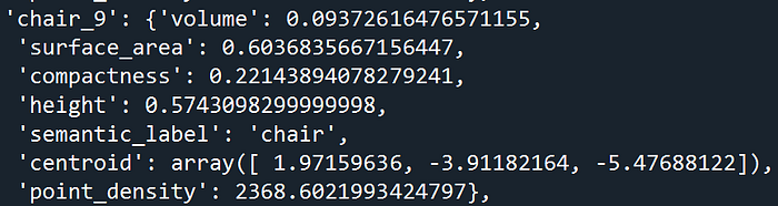
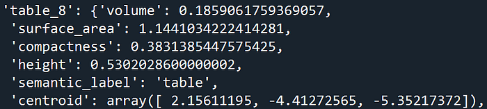
As you can see, the features for different classes are very different, which can give us additional spatial analytics workflows.

🌱 Growing Note: Add custom features for your domain. For furniture analysis, compute seat height, leg count, or symmetry measures. The feature dictionary is your canvas.

Now, we can move forward with the most structuring part: extracting relationships from our dataset.

Step 7. Spatial Relationship Computation + Topology

Spatial relationships emerge from geometric proximity and orientation analysis.

We want to build a system with spatial intelligence about when objects are above, below, adjacent, or contained within each other through 3D volume comparisons and distance thresholds.

Let us develop a set of functions to discover how objects relate to each other in space. Indeed, objects rarely exist in isolation.

Chairs cluster around tables. Lamps sit on surfaces. Walls define boundaries. We want a function that finds all these hidden connections.

For this, I propose a clever trick: a three-stage algorithm breakdown.

Stage 1: Topology analytics

I want to determine if one object is completely inside another, and if it is adjacent (Essential for hierarchical scene understanding.)

For object A to be contained in object B, all of A's boundaries must be within B's boundaries. This means we want to check all six faces (min/max for X, Y, Z):

def is_contained(bounds1, bounds2):
    """Check if object1 is contained within object2."""
    return (np.all(bounds1['min'] >= bounds2['min']) and 
            np.all(bounds1['max'] <= bounds2['max']))

Why This Works:

• bounds1['min'] >= bounds2['min']: Object 1's minimum corner is inside Object 2
• bounds1['max'] <= bounds2['max']: Object 1's maximum corner is inside Object 2
• np.all(): ALL three dimensions (X, Y, Z) must satisfy the condition

This is very simple, but beware that this is an axis-aligned bounding box containment check. It fails for rotated objects where the actual object is contained, but the bounding box isn't.

🌱 Growing Note: For rotated object containment, use oriented bounding boxes (OBB) or point-in-polygon tests with the actual object geometry.

Okay, what about determining when do objects touch or nearly touch?

We want to check if any face of one object is within tolerance distance of any face of the other object.

Each 3D "bounding-box" object has six faces (front/back, left/right, top/bottom). I check if any face pair is closer than the tolerance threshold:

def are_adjacent(bounds1, bounds2, tolerance=0.1):
    # Check if faces are close along each axis
    for axis in range(3):  # X, Y, Z axes
        # Face-to-face proximity checks
        if (abs(bounds1['max'][axis] - bounds2['min'][axis]) < tolerance or
            abs(bounds2['max'][axis] - bounds1['min'][axis]) < tolerance):
            return True
    return False

my logic is if bounds1['max'][axis] - bounds2['min'][axis] < tolerance, they're adjacent along this axis.

🦥 Florent's Geeky Note: The tolerance parameter handles measurement uncertainty and slight gaps between objects that appear to touch in real life.

I just make sure that I do all these tests to get an exhaustive description or relations and the basic 3D topology of our scene's objects.

🌱 Growing Note: Use different tolerance values for different object types. Walls might need 0.05m tolerance, while furniture could use 0.2m for "close enough" adjacency.

Beautiful. At this stage, we have already some clear ideas about a first-hand topology description. let us use these to classify our relationships.

Stage 2: Relationship Classification

For each nearby pair, we want to classify their spatial connection.

For that purpose, I propose to build a function that looks at two objects and determines their spatial relationship. Are they stacked? Adjacent? One inside the other?

Let us build determine_relationship_type(), to apply geometric tests to classify their relationship:

def determine_relationship_type(obj1, obj2, threshold):
    centroid1 = obj1['centroid']
    centroid2 = obj2['centroid']
    
    distance = np.linalg.norm(centroid1 - centroid2)
    if distance > threshold:
        return None  # Too far apart
    
    # Vertical relationship analysis
    z_diff = centroid1[2] - centroid2[2]
    if abs(z_diff) > 0.5:  # Significant height difference
        return 'above' if z_diff > 0 else 'below'
    
    # Containment analysis
    bounds1 = obj1['bounds']
    bounds2 = obj2['bounds']
    
    if is_contained(bounds1, bounds2):
        return 'inside'
    elif is_contained(bounds2, bounds1):
        return 'contains'
    
    # Adjacency analysis
    if are_adjacent(bounds1, bounds2, tolerance=0.3):
        return 'adjacent'
    
    return 'near'  # Default fallback

As you can see, I put a priority order of tests:

1. Distance Check: Too far apart? No relationship.
2. Vertical Analysis: Height differences indicate stacking relationships.
3. Containment Test: Is one object inside the other?
4. Adjacency Test: Do they share boundaries?
5. Fallback: Default to "near" if close but no specific relationship.

🦥 Ville's Geeky Note: The 0.5-meter vertical threshold works for typical indoor furniture heights. Adjust for your scale — smaller for tabletop scenes, larger for architectural analysis.

These are key in describing the relationships previously extracted.

🌱 Growing Note: Add semantic-aware relationship detection. A "lamp on table" relationship might need different geometric criteria than "book on table."

Now, let us move up the analytics a notch.

Stage 3: Exhaustive Pairwise Analysis

We are going to check every object against every other object.

For N objects, that's N×(N-1)/2 comparisons. This means that we can use the following function:

def compute_spatial_relationships(objects, distance_threshold=2.0):
    relationships = []
    object_names = list(objects.keys())
    
    for i, obj1 in enumerate(object_names):
        for j, obj2 in enumerate(object_names[i+1:], i+1):  # Avoid duplicates
            rel_type = determine_relationship_type(objects[obj1], objects[obj2], distance_threshold)
            if rel_type:  # Only keep valid relationships
                relationships.append((obj1, obj2, rel_type))
    
    return relationships

🦥 Geeky Note: The nested loop with enumerate(object_names[i+1:], i+1) ensures each pair is checked exactly once. No duplicate relationships.

what is intersting, is that you then get a very thorough relationship definition of our scene combining all the previous elements. However, if you deal with very large scenes (5M+ objects), consider spatial indexing (KD-trees) to avoid checking distant object pairs. The current O(N²) approach becomes slow.

On top, only objects within distance_threshold get relationship analysis. Far objects are ignored. as a guide for setting the value:

• 1.0–2.0: Intimate spatial relationships (touching, very close)
• 2.0–3.0: Functional relationships (chair near table)
• 3.0–5.0: Room-scale relationships (furniture groupings)
• 5.0+: Architectural relationships (across-room connections)

Now, we can start building our scene graph

Step 8. Building the Scene Graph

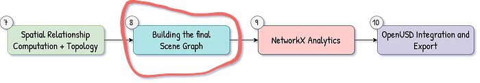
Let us focus on constructing the final NetworkX graph that represents our scene's spatial intelligence.

You have objects, relationships, and features scattered across different data structures. build_scene_graph() weaves them into a unified graph where nodes are objects and edges are spatial relationships:

def build_scene_graph(objects, relationships, features):
    G = nx.DiGraph()
    
    # Add nodes with rich attributes
    for obj_name, obj_data in objects.items():
        obj_features = features.get(obj_name, {}).copy()
        obj_features.pop('semantic_label', None)  # Avoid conflicts
        
        G.add_node(obj_name, 
                  semantic_label=obj_data['semantic_label'],
                  centroid=obj_data['centroid'].tolist(),
                  point_count=obj_data['point_count'],
                  **obj_features)
    
    # Add relationship edges
    for obj1, obj2, rel_type in relationships:
        G.add_edge(obj1, obj2, relationship=rel_type)
    
    return G

🦚 Florent's Note: The obj_features.pop('semantic_label', None) line prevents duplicate keyword arguments when adding nodes. NetworkX would crash on duplicate keys.

When designing our graph, we've opted for a directed graph due to the inherently directional nature of the relationships we're modeling. For instance, a table can support a lamp, but a lamp doesn't support a table;

Similarly, a room contains a chair, but a chair doesn't contain a room. This choice allows us to accurately represent these asymmetric and hierarchical connections within our 3D environment.

For our node attribute strategy, we'll store frequently accessed data like semantic_label and centroid directly on the nodes themselves for quick retrieval. However, larger datasets such as the raw point coordinates will be stored externally, with nodes holding only references to these external data, ensuring our graph remains efficient and lean for queries.

We'll also use consistent attribute naming conventions throughout to make navigating and querying the graph more straightforward.

🌱 Growing Note: Add edge weights based on relationship strength or confidence. This enables weighted graph algorithms for pathfinding and centrality analysis.

Node attributes store both geometric and semantic properties. Each object node contains its semantic label, spatial position, geometric features like volume and surface area, plus any custom attributes from your analysis pipeline.

🐦 Ville's Note: NetworkX stores all attributes in memory. For scenes with 1000+ objects, consider using node attribute factories or external storage for large data like point coordinates.

Edge attributes encode relationship semantics. The relationship type ("above," "adjacent," "contains") becomes queryable metadata that enables spatial reasoning queries later in your application.

🌱 Florent's Note: Rich node and edge attributes enable complex spatial queries. You can find all chairs near tables, objects above the floor level, or containers with specific contents — all through simple graph traversal.

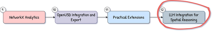
Step 9. NetworkX Analytics That Matter

Raw graphs are hard to understand. analyze_scene_graph() computes summary statistics that reveal the scene's spatial structure and complexity:

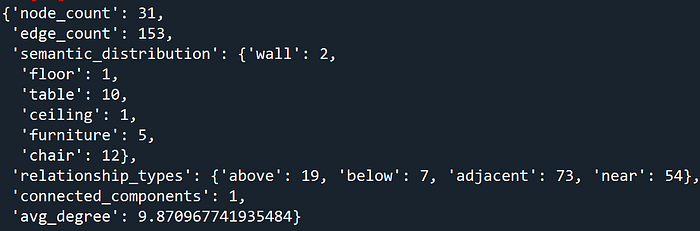
def analyze_scene_graph(G):
    analysis = {
        'node_count': G.number_of_nodes(),
        'edge_count': G.number_of_edges(),
        'semantic_distribution': {},
        'relationship_types': {},
        'connected_components': nx.number_weakly_connected_components(G),
        'avg_degree': sum(dict(G.degree()).values()) / G.number_of_nodes() if G.number_of_nodes() > 0 else 0
    }
    
    # Analyze semantic distribution
    for node, data in G.nodes(data=True):
        label = data.get('semantic_label', 'unknown')
        analysis['semantic_distribution'][label] = analysis['semantic_distribution'].get(label, 0) + 1
    
    # Analyze relationship types
    for _, _, data in G.edges(data=True):
        rel = data.get('relationship', 'unknown')
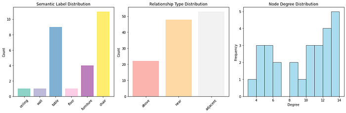
        analysis['relationship_types'][rel] = analysis['relationship_types'].get(rel, 0) + 1

Our algorithm meticulously computes several key metrics to provide a comprehensive understanding of the room's furniture graph:

It starts by determining node and edge counts, giving us a fundamental measure of the graph's overall size and complexity. Next, it analyzes the semantic distribution, revealing the prevalence of each object type, such as how many chairs versus tables are present.

The algorithm then identifies various relationship types, uncovering the specific spatial connections that exist between furniture pieces. Finally, it quantifies the connectivity of the scene, indicating how well-interconnected the objects are, and calculates the average degree, which tells us the typical number of relationships each object has within the graph.

🦥 Ville's Geeky Note: weakly_connected_components counts components in the underlying undirected graph. It tells you if your scene has isolated object clusters.

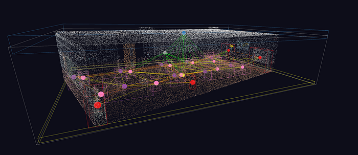
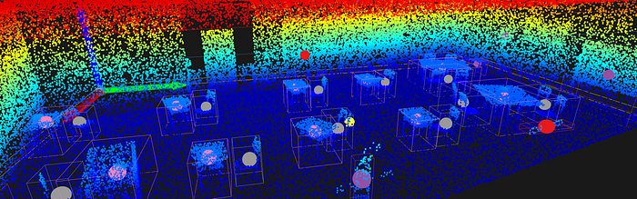
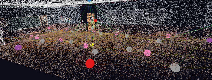
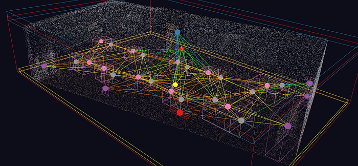
You can plot the graph in both 2D and 3D to get even deeper insights:

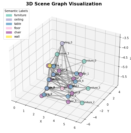
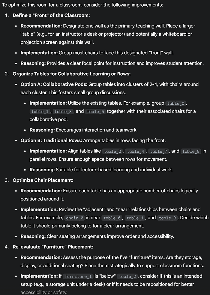
This room is currently configured with 31 objects, including 10 tables, 12 chairs, 5 pieces of furniture, 2 walls, a ceiling, and a floor.

The dominant relationships between objects are "adjacent" and "near," suggesting a scattered arrangement of individual or small seating areas rather than a unified setup.

The high average degree of connections between objects (9.94) further indicates a dense and interconnected environment without a clear focal point for a classroom setting.

🌱 Growing Note: Add domain-specific metrics like "seating capacity" (count chairs), "workspace count" (desk+chair combinations), or "accessibility score" (path length analysis).

[BONUS] Advanced Scene Graph Pattern Matching

The hardest part of spatial intelligence isn't finding objects.

It's finding meaningful patterns that repeat across complex environments. You've built scene graphs for individual rooms, but what happens when you need to find every "meeting space" or "workstation setup" across an entire building complex?

Traditional object detection tells you "here's a chair, here's a table." But pattern matching reveals "here's a collaborative workspace with optimal sight lines" or "here's a presentation area with proper audience orientation."

This transforms your scene graphs from simple object catalogs into intelligent spatial pattern detectors that understand how spaces function.

The Pattern Recognition Challenge

Large building complexes contain thousands of objects arranged in recurring functional patterns.

Meeting rooms share similar spatial signatures — tables surrounded by chairs, often with presentation equipment nearby. Workstations cluster desks with task chairs and storage. Reception areas combine seating arrangements with service counters.

Your scene graph contains all this spatial intelligence, but finding these patterns manually would require checking every possible object combination.

For a building with 10,000 objects, that's computationally impossible.

NetworkX provides the solution through subgraph isomorphism — automatically detecting when smaller pattern graphs appear within larger scene graphs.

🦚 Florent's Note: This approach draws from computer vision's template matching, but applies it to spatial relationships rather than pixel patterns. The referenced paper by Yue et al. demonstrates how 3D scene graphs enable robust indoor scene recognition at building scale.

Building Pattern Detection Functions

Subgraph isomorphism finds exact matches between pattern and scene graphs, but real-world spaces have variations.

Your pattern matching system needs flexibility to handle different chair arrangements around similar table configurations, or presentation setups with varying equipment layouts.

This requires custom matching functions that understand semantic equivalence. The core matching engine uses NetworkX's DiGraphMatcher with custom comparison functions such as:

def create_pattern_matcher(scene_graph, pattern_graph, 
                          node_attr='semantic_label', 
                          edge_attr='relationship'):
    """Create flexible pattern matcher for scene graph analysis."""
    
    def semantic_node_match(node1_attrs, node2_attrs):
        """Check if nodes match semantically with flexibility."""
        label1 = node1_attrs.get(node_attr, 'unknown')
        label2 = node2_attrs.get(node_attr, 'unknown')
        
        # Exact match first
        if label1 == label2:
            return True
            
        # Semantic equivalence groups
        furniture_group = {'chair', 'seat', 'stool'}
        surface_group = {'table', 'desk', 'surface'}
        
        if label1 in furniture_group and label2 in furniture_group:
            return True
        if label1 in surface_group and label2 in surface_group:
            return True
            
        return False
    
    def relationship_edge_match(edge1_attrs, edge2_attrs):
        """Check if relationships match with spatial tolerance."""
        rel1 = edge1_attrs.get(edge_attr, 'unknown')
        rel2 = edge2_attrs.get(edge_attr, 'unknown')
        
        # Direct match
        if rel1 == rel2:
            return True
            
        # Spatial relationship equivalence
        proximity_group = {'adjacent', 'near', 'close'}
        support_group = {'above', 'on', 'supported_by'}
        
        if rel1 in proximity_group and rel2 in proximity_group:
            return True
        if rel1 in support_group and rel2 in support_group:
            return True
            
        return False
    
    # Create NetworkX matcher with custom comparison functions
    matcher = nx.algorithms.isomorphism.DiGraphMatcher(
        scene_graph,
        pattern_graph,
        node_match=semantic_node_match,
        edge_match=relationship_edge_match
    )
    
    return matcher

The semantic matching functions handle real-world variations while maintaining pattern recognition accuracy.

Node matching groups similar furniture types, while edge matching recognizes equivalent spatial relationships.

This flexibility allows your pattern detector to find "meeting spaces" regardless of whether they use chairs or stools, tables or desks, as long as the spatial arrangement matches the functional pattern.

🐦 Ville's Note: The DiGraphMatcher uses the VF2 algorithm internally, which has exponential worst-case complexity but performs well on sparse graphs typical of spatial scenes. The semantic groupings reduce false negatives while maintaining precision.

Pattern Definition and Detection

Real pattern detection requires defining what you're searching for through example scene graphs.

Meeting room patterns typically contain a central surface surrounded by seating, often with additional equipment nearby. Workstation patterns show individual work surfaces with associated seating and storage. Each pattern becomes a small scene graph that captures the essential spatial relationships.

def create_meeting_room_pattern():
    """Define meeting room spatial pattern as scene graph."""
    pattern = nx.DiGraph()
    
    # Core meeting room components
    pattern.add_node('table_1', semantic_label='table')
    pattern.add_node('chair_1', semantic_label='chair')
    pattern.add_node('chair_2', semantic_label='chair')
    pattern.add_node('chair_3', semantic_label='chair')
    
    # Spatial relationships
    pattern.add_edge('chair_1', 'table_1', relationship='adjacent')
    pattern.add_edge('chair_2', 'table_1', relationship='adjacent')
    pattern.add_edge('chair_3', 'table_1', relationship='adjacent')
    
    return pattern

def create_workstation_pattern():
    """Define individual workstation spatial pattern."""
    pattern = nx.DiGraph()
    
    # Workstation components
    pattern.add_node('desk_1', semantic_label='desk')
    pattern.add_node('chair_1', semantic_label='chair')
    pattern.add_node('storage_1', semantic_label='furniture')
    
    # Functional relationships
    pattern.add_edge('chair_1', 'desk_1', relationship='adjacent')
    pattern.add_edge('storage_1', 'desk_1', relationship='near')
    
    return pattern
def find_spatial_patterns(scene_graph, pattern_graph):
    """Find all occurrences of pattern within scene graph."""
    matcher = create_pattern_matcher(scene_graph, pattern_graph)
    
    matches = list(matcher.subgraph_isomorphisms_iter())
    
    # Extract match details with spatial context
    pattern_matches = []
    for match in matches:
        # match maps pattern nodes to scene nodes
        scene_objects = list(match.values())
        
        # Calculate pattern centroid for spatial reference
        centroids = []
        for obj_id in scene_objects:
            if scene_graph.has_node(obj_id):
                centroid = scene_graph.nodes[obj_id].get('centroid', [0,0,0])
                centroids.append(centroid)
        
        if centroids:
            pattern_center = np.mean(centroids, axis=0)
            pattern_matches.append({
                'objects': scene_objects,
                'mapping': match,
                'center': pattern_center.tolist(),
                'confidence': calculate_pattern_confidence(scene_graph, match)
            })
    
    return pattern_matches
def calculate_pattern_confidence(scene_graph, node_mapping):
    """Calculate confidence score for pattern match."""
    confidence_factors = []
    
    # Geometric consistency
    positions = []
    for scene_node in node_mapping.values():
        centroid = scene_graph.nodes[scene_node].get('centroid', [0,0,0])
        positions.append(centroid)
    
    if len(positions) > 1:
        # Measure spatial compactness
        distances = []
        for i, pos1 in enumerate(positions):
            for pos2 in positions[i+1:]:
                distances.append(np.linalg.norm(np.array(pos1) - np.array(pos2)))
        
        avg_distance = np.mean(distances)
        # Lower average distance = higher confidence for compact patterns
        spatial_confidence = max(0, 1.0 - avg_distance / 5.0)  # 5m normalization
        confidence_factors.append(spatial_confidence)
    
    # Semantic consistency (could add more factors)
    semantic_confidence = 1.0  # Placeholder for semantic validation
    confidence_factors.append(semantic_confidence)
    
    return np.mean(confidence_factors)

The pattern detection system returns detailed matches with spatial context and confidence scores. This enables filtering weak matches and ranking results by spatial quality.

Each detected pattern includes the specific objects involved, their spatial arrangement, and a confidence measure based on geometric consistency and semantic coherence.

🌱 Growing Note: Extend pattern libraries for domain-specific applications. Healthcare facilities need patterns for examination rooms and nursing stations. Retail spaces require checkout configurations and product displays. Each domain has characteristic spatial signatures that pattern matching can detect automatically.

The pattern-matching approach scales to building complexes by processing individual room scene graphs and aggregating pattern discoveries across spaces.

This enables facility management queries like "find all underutilized meeting rooms" or "identify non-standard workstation configurations."

You can check out this paper to get more insights:

Yue, H., Lehtola, V., Wu, H., Vosselman, G., Li, J., & Liu, C. (2024). Recognition of Indoor Scenes using 3D Scene Graphs. IEEE Transactions on Geoscience and Remote Sensing.

Below is a generic, reusable helper that allows you to search any large scene graph (E.g., a building) for occurrences of another small scene graph (E.g., a place described with a scene graph).

matcher = nx.algorithms.isomorphism.DiGraphMatcher(
        G,
        pattern,
        node_match=lambda d1, d2: node_cmp(d1.get(node_attr), d2.get(node_attr)),
        edge_match=lambda d1, d2: edge_cmp(d1.get(edge_attr), d2.get(edge_attr)),
    )

    # NetworkX streams one mapping at a time
    yield from matcher.subgraph_isomorphisms_iter()

🐦 Ville's note: The helper relies on NetworkX's built-in subgraph-isomorphism engine and works with the attribute conventions you have already adopted (semantic_label on nodes, relationship on edges).

Step 10. OpenUSD Integration and Export

USD transforms your scene graph into an industry-standard format.

OpenUSD provides a schema for encoding semantic relationships and geometric properties in a manner that production pipelines can understand. Your NetworkX graph becomes a hierarchical USD stage with proper primitive organization.

The export process creates USD primitives for each object, assigns semantic attributes, and encodes spatial relationships as stage metadata.

• Step 1: Create USD Stage. Initialize a new USD stage (think "empty movie set").
• Step 2: Establish Scene Hierarchy. Create an organized structure: Scene root → Geometry scope → Individual objects.
• Step 3: Add Object Primitives. Each scene graph node becomes a USD primitive (cube placeholder) with semantic attributes.
• Step 4: Encode Relationships. Store spatial relationships as stage metadata for downstream applications.

This can be done with this function:

def create_usd_stage(scene_graph: nx.DiGraph, output_path: str) -> bool:
    """Create USD stage from scene graph and export to file."""
    if not USD_AVAILABLE:
        print("USD not available. Cannot create USD stage.")
        return False
    
    # Create new stage
    stage = Usd.Stage.CreateNew(output_path)
    
    # Set up scene hierarchy
    root_prim = stage.DefinePrim('/Scene', 'Xform')
    stage.SetDefaultPrim(root_prim)
    
    # Create geometry scope for objects
    geom_scope = UsdGeom.Scope.Define(stage, '/Scene/Geometry')
    
    # Add each object as a primitive
    for node, data in scene_graph.nodes(data=True):
        create_usd_object(stage, node, data)
    
    # Add relationships as metadata
    add_relationships_to_stage(stage, scene_graph)
    
    # Save stage
    stage.Save()
    return True

Each object is converted into a USD primitive with semantic attributes attached. The system uses cube primitives as placeholders, but you can extend this to use proper geometry from your point cloud data.

Spatial relationships get encoded as stage metadata rather than USD relationships. This approach preserves the relationship information while maintaining compatibility with standard USD workflows.

/Scene (Root Transform)
├── /Scene/Geometry (Scope for objects)
│   ├── Chair_1 (Cube primitive + attributes)
│   ├── Table_1 (Cube primitive + attributes)
│   └── Lamp_1 (Cube primitive + attributes)
└── Metadata (Relationship information)

🦥 Florent's Geeky Note: USD stages use hierarchical organization with scopes and transforms. The /Scene/Geometry scope contains all object primitives, while relationships live as root-level metadata for easy access. We use Cube prims as geometric placeholders, but you could substitute actual mesh geometry from the point clouds.

From there, where can we go?

Step 11. Practical Applications and Extensions

Scene graphs unlock spatial intelligence across industries.

The modular pipeline design enables domain-specific extensions.

You can add physics properties for simulation, temporal relationships for dynamic scenes, or custom semantic hierarchies for specialized applications.

Performance scales linearly with point cloud size for most operations.

DBSCAN clustering and distance computations dominate processing time; however, parallel processing and spatial indexing can accelerate processing of large datasets.

Here is a pipeline view of the process:

def process_semantic_pointcloud_to_usd(input_path, output_usd, eps = 0.8, min_samples = 15, distance_threshold = 3.0):
    """Complete pipeline from semantic point cloud to USD scene graph."""
    results = {'success': False, 'files_created': [], 'analysis': {}}
    
    try:
        # Load and validate data
        print("Loading semantic point cloud...")
        df = load_semantic_point_cloud(input_path)
        
        print(f"Loaded {len(df)} points with {df['semantic_label'].nunique()} semantic classes")
        
        # Extract objects
        print("Extracting semantic objects...")
        objects = extract_semantic_objects(df, eps=eps, min_samples=min_samples)
        print(f"Found {len(objects)} objects")
        
        # Compute features
        print("Computing object features...")
        features = compute_object_features(objects)
        
        # Find relationships
        print("Computing spatial relationships...")
        relationships = compute_spatial_relationships(objects, distance_threshold)
        print(f"Found {len(relationships)} spatial relationships")
        
        # Build scene graph
        print("Building scene graph...")
        scene_graph = build_scene_graph(objects, relationships, features)
        
        # Validate scene graph
        validation = validate_scene_graph(scene_graph)
        if not validation['is_valid']:
            print("Warning: Scene graph validation found issues:", validation['issues'])
        
        # Export to USD
        if USD_AVAILABLE:
            print(f"Exporting to USD: {output_usd}")
            usd_success = create_usd_stage(scene_graph, output_usd)
            if usd_success:
                results['files_created'].append(output_usd)
        
        # Export summary
        summary_path = output_usd.replace('.usda', '_summary.json')
        export_scene_summary(scene_graph, summary_path)
        results['files_created'].append(summary_path)
        
        # Store analysis results
        results['analysis'] = analyze_scene_graph(scene_graph)
        results['validation'] = validation
        results['success'] = True
        
        print("Pipeline completed successfully!")
        
    except Exception as e:
        print(f"Pipeline failed: {str(e)}")
        results['error'] = str(e)
    
    return results

The complete pipeline processes semantic point clouds end-to-end. Error handling and validation ensure robust operation across different data sources and formats.

# Complete pipeline execution
process_semantic_pointcloud_to_usd('../DATA/indoor_room_labelled.csv', 'demo_scene_c.usda', eps = 0.2, min_samples = 20, distance_threshold = 3.0)

Integration with existing 3D pipelines happens through standard USD workflows. Your scene graphs become first-class assets in production environments, queryable through standard USD tools and APIs.

🐦 Ville's Note: Consider extending the pipeline with temporal relationships for dynamic scenes, physics properties for simulation, or custom ontologies for domain-specific semantic hierarchies.

Step 12. LLM Integration for Spatial Reasoning

Scene graphs become powerful when connected to large language models.

Your structured spatial data transforms into natural language queries that LLMs can understand and reason about.

Instead of complex geometric calculations, you can ask questions like "find all chairs near windows" or "identify cluttered areas in the room."

The key is converting your NetworkX scene graph into text representations that preserve spatial relationships.

LLMs like Mistral, DeepSeek, or GPT can then apply their reasoning capabilities to your 3D scene understanding. This is what we could achieve:

Modern LLMs excel at analyzing relationships and making logical inferences. When you provide them with structured scene descriptions, they can identify patterns, answer spatial queries, and even suggest optimizations for space usage.

def query_scene_with_llm(scene_graph: nx.DiGraph, user_question: str, 
                        llm_client=None) -> str:
    """Query scene graph using LLM reasoning capabilities."""
    
    # Create structured scene description
    scene_context = scene_graph_to_llm_prompt(scene_graph)
    
    # Build complete prompt
    full_prompt = f"""{scene_context}

USER QUESTION: {user_question}
Please provide a detailed answer based on the spatial relationships and object positions in the scene. Consider:
1. Direct spatial relationships between objects
2. Accessibility and navigation paths
3. Functional groupings and usage patterns
4. Safety or optimization concerns

Users can ask natural language questions about room layout, furniture arrangement, or accessibility without needing to understand graph theory or 3D coordinates. Here is an example:

This approach works particularly well with models trained on spatial reasoning tasks. The structured prompt format helps LLMs understand the scene context while preserving the precision of your geometric analysis.

🦥 Our Geeky Note: The prompt structure includes object positions, semantic labels, and relationship types in a format that LLMs can parse effectively. Temperature settings around 0.3–0.7 work well for spatial reasoning tasks — low enough for accuracy, high enough for creative insights.

Conclusion

Scene graphs bridge the gap between raw 3D data and spatial intelligence.

This tutorial showed you how to extract semantic objects from point clouds, compute spatial relationships, and encode everything into OpenUSD format.

The techniques scale from single rooms to complex environments. Your semantic point clouds become queryable knowledge bases, enabling the next generation of spatial AI applications.

you can now handle real-world complexity while maintaining production-ready performance. Each component operates independently, allowing customization without breaking the overall workflow.

You can apply this pipeline to your semantic point cloud data.

Start with the sample data generator to understand the workflow, then process your real datasets.

The combination of scene graphs and OpenUSD will undoubtedly unlock spatial intelligence that traditional 3D formats cannot provide. This allows you to generate a complete software like this one:

🦚Florent Poux, Ph.D.: The true ingenuity of this tutorial is not the technical steps of converting raw point cloud data into structured 3D scene graphs, but in its profound implications for spatial intelligence. Critically, it highlights a paradigm shift: we're moving beyond the visualization of 3D geometry to creating dynamically queryable knowledge bases. This fusion of computational geometry with graph theory (think NetworkX's elegant graph representations) and the semantic power of LLMs via OpenUSD is a geeky triumph.

🐦Ville's Note: It's a testament to how data abstraction and precise orchestration of diverse algorithmic components — from DBSCAN's clustering to spatial relationship inference — can unlock autonomous systems to perceive and reason about 3D environments with human-like understanding, fundamentally altering our interaction with digital twins and beyond.

📦 Resources

Here's a curated list of references that I recommend for deepening your understanding of the techniques we've covered:

I created a special standalone episode, accessible in this Open-Access Course. You will find:

1. The complete tutorial with under-the-hood tricks📜
2. The whole dataset to download️
3. The code implementation with a permissive license💻
4. Additional resources (cheat sheet, paper …)🌍

🦚Florent: This is all offered 🎁, and based on the book above. Feel free to get it to support this knowledge sharing initiative.

3D Scene Graphs & LLM Integration

• SG-Nav: Online 3D Scene Graph Prompting for LLM-based Zero-shot Object Navigation by NIPS: An academic paper exploring hierarchical 3D scene graphs for LLM-based navigation. SG-Nav Paper
• Open3DSG: Open-Vocabulary 3D Scene Graphs from Point Clouds with Queryable Objects and Open-Set Relationships by arXiv: A research paper on creating open-vocabulary 3D scene graphs from point clouds. Open3DSG Paper
• 3DGraphLLM: Combining Semantic Graphs and Large Language Models for 3D Scene Understanding by arXiv: Another academic paper on constructing learnable representations of 3D scene graphs for LLM input. 3DGraphLLM Paper
• Enhancing Language Models' Understanding of 3D Environments through Scene Graphs by kth.diva: A thesis investigating how scene graphs can bridge the gap between 3D scenes and large language models. Enhancing LLMs Understanding Paper

NetworkX Documentation

• NetworkX Official Documentation: The primary resource for the NetworkX Python package, including tutorials and reference guides. NetworkX Documentation
• NetworkX Tutorial: A comprehensive tutorial on using NetworkX for graph creation, manipulation, and analysis. NetworkX Tutorial

OpenUSD Documentation & Resources

• How to Use OpenUSD | NVIDIA Technical Blog: An introduction to Universal Scene Description (OpenUSD) with essential concepts and best practices. How to Use OpenUSD
• Universal Scene Description (OpenUSD) GitHub Repository: The official GitHub repository for OpenUSD by Pixar Animation Studios, containing source code and additional documentation. OpenUSD GitHub

For those looking to apply these concepts professionally, check out my comprehensive 3D Segmentor OS course. It expands on these foundations with production-ready code and advanced techniques I've developed through years of real-world projects.

About the authors

Florent Poux, Ph.D. is a Scientific and Course Director focused on educating engineers on leveraging AI and 3D Data Science. He leads research teams and teaches 3D Computer Vision at various universities. His current aim is to ensure humans are correctly equipped with the knowledge and skills to tackle 3D challenges for impactful innovations.

— — — —

Dr. Ville Lehtola is Assistant Professor in the Earth Observation Science (EOS) Department at ITC faculty of the University of Twente. The topic of his professorship is 'indoor and mobile mapping'. He is also Associate Professor (Dosentti) in "Computational Science, especially Multi-Sensor Fusion and Machine Learning" at Faculty of Information Sciences, University of Jyväskylä, Finland.